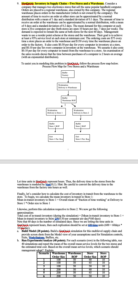
9. SivaQuicks: Inventory in Supply Chains --Two Stores and a Warehouse. Consider a company that manages two electronics stores that sell the same popular handheld computer. Orders are placed to a regional warehouse, also owned by this company. The regional warehouse places orders to the manufacturer (which is not owned by the company). The amount of time to receive an order at either store can be approximated by a normal distribution with a mean of 1 day and a standard deviation of 0.1 days. The amount of time to receive an order at the warehouse can be approximated by a normal distribution, with a mean of 4 days and a standard deviation of 0.2 days. The mean demand for this computer at each store is five computers per day (both stores are open 10 hours per day, 7 days per week). The demand is expected to remain the same at both stores for the next 60 days. Management wants to use a reorder point scheme at the stores and the warehouse. Their goal is to achieve at least a 95% service level at each store at minimum cost. The ordering costs are $75 every time a store places an order to the warehouse and $150 every time the warehouse places an order to the factory. It also costs $0.50 per day for every computer in inventory at a store, and $0.10 per day for every computer in inventory at the warehouse. We assume it also costs $0.10 per day for every computer in transit from the warehouse to a store. An examination of the sales records shows that the time between purchases of a computer is 2 hours on average (with an exponential distribution). To assist you in modeling this problem in Sio Quick, follow the process flow map below. Process Flow Map for Two Stores and a Warehouse Buffer Factory Workstation Delivery to Warehouse Buffer Warehouse ROP 1 Workstation Delivery to Store Workstation Delivery to Store 2 Buffer Store 1 ROP Buffer Store 2 ROP Exit Store Pur. Req. Exit Store 2 Pur, Rey Let time units in SiwQuick represent hours. Thus, the delivery time to the stores from the warehouse is modeled by No: 10,1). Hint: Be careful to convert the delivery time to the warehouse from the factory into hours as well. Finally, let's consider how to calculate the cost of inventory in transit from the warehouse to the store. To begin, we calculate the mean inventory in transit to Store 1: Mean in-transit inventory to Store 1 - Overall mean of "fraction of time working" at Delivery to Store 1 Order size to Store 1 Likewise, perform this calculation respective to Store 2. We now get the following approximation: Total : cost of in-transit inventory (during the simulation) - [Mean in-transit inventory to Store 1 + Mean in-transit inventory to Store 20.50 per computer per day)*(60 days) Note that 60 days is the number of simulated days. Since we are letting the time units in SiwQuick represent hours, then each replication should be set at 6 time units (600 - 60days 10 bus day). a. Build Model (28 points). Build a Sio Quick simulation for this multilevel supply chain and provide screen shots from the Model view of your assumptions used for Simulation controls, Exits, Werle Station. Buffers, etc. b. Run Experiments/Analyze (48 points). For each scenario (row) in the following table, run 40 simulations and report the mean of the overall mean service levels for the two stores and the estimated total cost. Based on the overall mean service levels, which scenario should management adopt? Explain. Scenario Warehouse Warehouse Store Store Order Size ROP Order Size ROP 100 50 40 10 100 45 10 50 10 4 50 40 200 45 10 2002 50 50 1002 50 50 100 200 10 50 9. SivaQuicks: Inventory in Supply Chains --Two Stores and a Warehouse. Consider a company that manages two electronics stores that sell the same popular handheld computer. Orders are placed to a regional warehouse, also owned by this company. The regional warehouse places orders to the manufacturer (which is not owned by the company). The amount of time to receive an order at either store can be approximated by a normal distribution with a mean of 1 day and a standard deviation of 0.1 days. The amount of time to receive an order at the warehouse can be approximated by a normal distribution, with a mean of 4 days and a standard deviation of 0.2 days. The mean demand for this computer at each store is five computers per day (both stores are open 10 hours per day, 7 days per week). The demand is expected to remain the same at both stores for the next 60 days. Management wants to use a reorder point scheme at the stores and the warehouse. Their goal is to achieve at least a 95% service level at each store at minimum cost. The ordering costs are $75 every time a store places an order to the warehouse and $150 every time the warehouse places an order to the factory. It also costs $0.50 per day for every computer in inventory at a store, and $0.10 per day for every computer in inventory at the warehouse. We assume it also costs $0.10 per day for every computer in transit from the warehouse to a store. An examination of the sales records shows that the time between purchases of a computer is 2 hours on average (with an exponential distribution). To assist you in modeling this problem in Sio Quick, follow the process flow map below. Process Flow Map for Two Stores and a Warehouse Buffer Factory Workstation Delivery to Warehouse Buffer Warehouse ROP 1 Workstation Delivery to Store Workstation Delivery to Store 2 Buffer Store 1 ROP Buffer Store 2 ROP Exit Store Pur. Req. Exit Store 2 Pur, Rey Let time units in SiwQuick represent hours. Thus, the delivery time to the stores from the warehouse is modeled by No: 10,1). Hint: Be careful to convert the delivery time to the warehouse from the factory into hours as well. Finally, let's consider how to calculate the cost of inventory in transit from the warehouse to the store. To begin, we calculate the mean inventory in transit to Store 1: Mean in-transit inventory to Store 1 - Overall mean of "fraction of time working" at Delivery to Store 1 Order size to Store 1 Likewise, perform this calculation respective to Store 2. We now get the following approximation: Total : cost of in-transit inventory (during the simulation) - [Mean in-transit inventory to Store 1 + Mean in-transit inventory to Store 20.50 per computer per day)*(60 days) Note that 60 days is the number of simulated days. Since we are letting the time units in SiwQuick represent hours, then each replication should be set at 6 time units (600 - 60days 10 bus day). a. Build Model (28 points). Build a Sio Quick simulation for this multilevel supply chain and provide screen shots from the Model view of your assumptions used for Simulation controls, Exits, Werle Station. Buffers, etc. b. Run Experiments/Analyze (48 points). For each scenario (row) in the following table, run 40 simulations and report the mean of the overall mean service levels for the two stores and the estimated total cost. Based on the overall mean service levels, which scenario should management adopt? Explain. Scenario Warehouse Warehouse Store Store Order Size ROP Order Size ROP 100 50 40 10 100 45 10 50 10 4 50 40 200 45 10 2002 50 50 1002 50 50 100 200 10 50