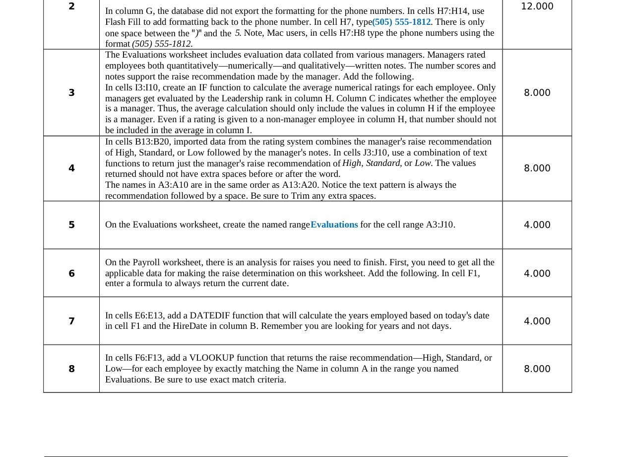
In column G, the database did not export die formatting for the phone numbers. In cells H7:H14, use Flash Fill to add formatting back to the phone number. In cell H7, type(505) 5554812. There is only one space between the ")" and the 5. Note, Mac users, in cells H7:H8 type the phone numbers using the format 505 555-1812. The Evaluations worksheet includes evaluation data collated from various managers. Managers rated employees both quantitativelynumericallyand qualitativelywritten notes. The number scores and notes support the raise recommendation made by the manager. Add the following. In cells 13:110, create an [F function to calculate the average numerical ratings for each employee. Only managers get evaluated by the Leadership rank in column H. Column C indicates whether the employee is a manager. Thus, the average calculation should only include the values in column H if the employee is a manager. Even if a rating is given to a non~manager employee in column H, that number should not be included in the average in column I. In cells B13:B20, imported data from the rating system combines the manager's raise recommendation of High, Standard, or Low followed by the manager's notes. In cells J3:J10, use a combination of text functions to retum just the manager's raise reconunendation of High, Standard, or Low. The values returned should not have extra spaces before or after die word. The names in A31A10 are in the same order as A13:A20. Notice the text pattern is always the reconu'nendation followed b a snace. Be sure to Trim an extra snaces. On the Evaluations worksheet, create the named rangeEvaluations for the cell range A3:J 10. On the Payroll worksheet, there is an analysis for raises you need to nish. First, you need to get all the applicable data for making the raise determination on this worksheet. Add the following. In cell F1, enter a formula to always return the current date. 12.000 8.000 8.000 4.000 4.000 In cells E6:E13, add a DATEDIF function that will calculate the years employed based on today's date in cell F1 and the HireDate in colunm B. Remember you are looking for years and not days. In cells F6:F13, add a VLOOKUP funcan that returns the raise recommendaonil-Iigh, Standard, or Lowfor each employee by exactly matching the Name in column A in the range you named Evaluations. Be sure to use exact match criteria. 4.000 8.000