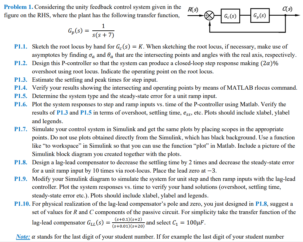
Problem 1. Considering the unity feedback control system given in the figure on the RHS, where the plant has the following transfer function, Gp(s)=s(s+7)1 P1.1. Sketch the root locus by hand for Gc(s)=K. When sketching the root locus, if necessary, make use of asymptotes by finding a and a that are the intersecting points and angles with the real axis, respectively. P1.2. Design this P-controller so that the system can produce a closed-loop step response making (2)% overshoot using root locus. Indicate the operating point on the root locus. P1.3. Estimate the settling and peak times for step input. P1.4. Verify your results showing the intersecting and operating points by means of MATLAB rlocus command. P1.5. Determine the system type and the steady-state error for a unit ramp input. P1.6. Plot the system responses to step and ramp inputs vs. time of the P-controller using Matlab. Verify the results of P1.3 and P1.5 in terms of overshoot, settling time, ess, etc. Plots should include xlabel, ylabel and legends. P1.7. Simulate your control system in Simulink and get the same plots by placing scopes in the appropriate points. Do not use plots obtained directly from the Simulink, which has black background. Use a function like "to workspace" in Simulink so that you can use the function "plot" in Matlab. Include a picture of the Simulink block diagram you created together with the plots. P1.8. Design a lag-lead compensator to decrease the settling time by 2 times and decrease the steady-state error for a unit ramp input by 10 times via root-locus. Place the lead zero at 3. P1.9. Modify your Simulink diagram to simulate the system for unit step and then ramp inputs with the lag-lead controller. Plot the system responses vs. time to verify your hand solutions (overshoot, settling time, steady-state error etc.). Plots should include xlabel, ylabel and legends. P1.10. For physical realization of the lag-lead compensator's pole and zero, you just designed in P1.8, suggest a set of values for R and C components of the passive circuit. For simplicity take the transfer function of the lag-lead compensator GLL(s)=(s+0.01)(s+20)(s+0.1)(s+2) and select C1=100F. Note: stands for the last digit of your student number. If for example the last digit of your student number