All Matches

Solution Library

Expert Answer

Textbooks

Search Textbook questions, tutors and Books

Oops, something went wrong!

Change your search query and then try again

Result Not Found

Books FREE
Tutors
Study Help
Ask a Question

Search
Sign In
Register

study help
mathematics
numerical analysis

Questions and Answers of Numerical Analysis

Suppose that N (h) is an approximation to M for every h > 0 and that M = N(h) + K1h + K2h2 + K3h3 +· · · , For some constants K1, K2, K3 . . . Use the values N (h), N (h/3) and N (h/9) to
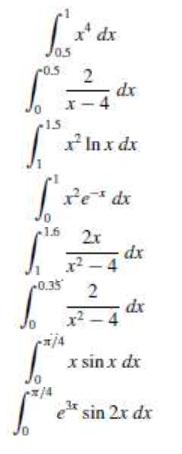
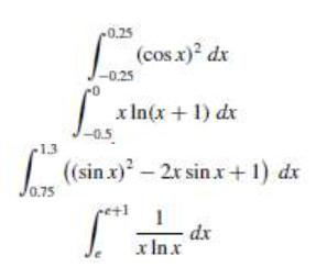
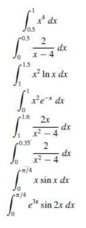
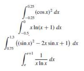
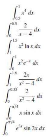
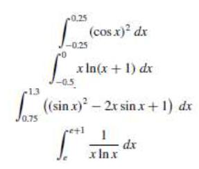
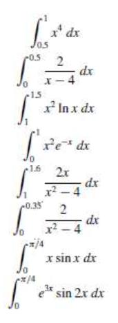
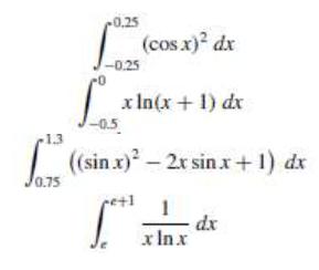
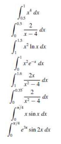
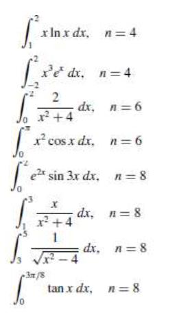
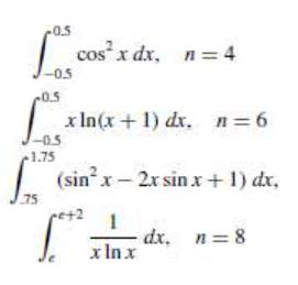
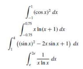
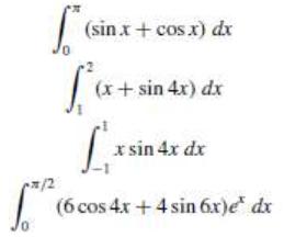
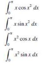
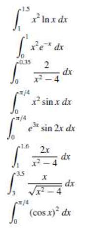
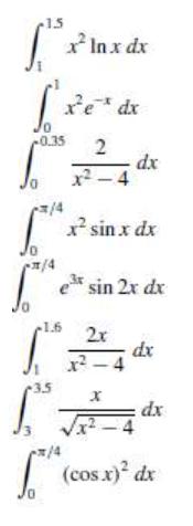
Approximate the following integrals using the Trapezoidal rule.
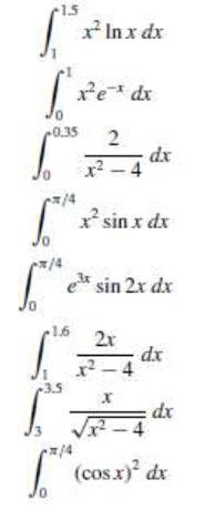
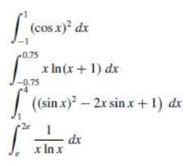
Repeat Exercise 2 using the Midpoint rule.In Exercise 2
Repeat Exercise 3 using the Midpoint rule and the results of Exercise 9.In Exercise 1
Repeat Exercise 4 using the Midpoint rule and the results of Exercise 10.In Exercise 2
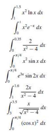
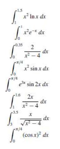
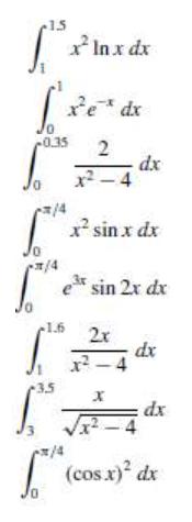
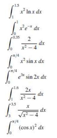
Approximate the following integrals using the Trapezoidal rule.
Approximate the following integrals using formulas (4.25) through (4.32). Are the accuracies of the approximations consistent with the error formulas? Which of parts (d) and (e) give the better
Given the function f at the following values,ApproximateUsing all the appropriate quadrature formulas of this section
Suppose that the data of Exercise 22 have round-off errors given by the following table.Calculate the errors due to round-off in Exercise 22.
Derive Simpson's rule with error term by usingFind a0, a1, and a2 from the fact that Simpson's rule is exact for f (x) = xn when n = 1, 2, and 3. Then find k by applying the integration formula with
Prove the statement following Definition 4.1; that is, show that a quadrature formula has degree of precision n if and only if the error E(P(x)) = 0 for all polynomials P(x) of degree k = 0, 1, . . .
Derive Simpson's three-eighths rule (the closed rule with n = 3) with error term by using Theorem 4.2.
Find a bound for the error in Exercise 1 using the error formula, and compare this to the actual error.In Exercise 1
Find a bound for the error in Exercise 2 using the error formula, and compare this to the actual error.In Exercise 2
Repeat Exercise 1 using Simpson's rule.In Exercise 1
Repeat Exercise 2 using Simpson's rule.In Exercise 2
Repeat Exercise 3 using Simpson's rule and the results of Exercise 5.In Exercise 3
Repeat Exercise 4 using Simpson's rule and the results of Exercise 6.In Exercise 4
Repeat Exercise 1 using the Midpoint rule.In Exercise 1
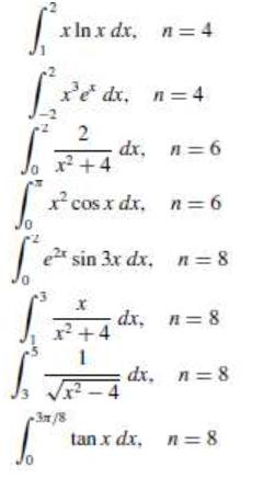
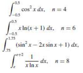
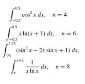
Use the Composite Trapezoidal rule with the indicated values of n to approximate the following integrals.
Determine the values of n and h required to approximateTo within 10ˆ’4 Usea. Composite Trapezoidal rule.b. Composite Simpson's rule.c. Composite Midpoint rule.
Repeat Exercise 11 for the integralIn Exercise 11Determine the values of n and h required to approximateTo within 10ˆ’4 Usea. Composite Trapezoidal rule.b. Composite Simpson's rule.c. Composite
Determine the values of n and h required to approximateTo within 10ˆ’5 and compute the approximation. Usea. Composite Trapezoidal rule.b. Composite Simpson's rule.c. Composite Midpoint rule.
Repeat Exercise 13 for the integralIn Exercise 13Determine the values of n and h required to approximateTo within 10ˆ’5 and compute the approximation. Usea. Composite Trapezoidal rule.b. Composite
Let f be defined bya. Investigate the continuity of the derivatives of f .b. Use the Composite Trapezoidal rule with n = 6 to approximateand estimate the error using the error bound.c. Use the
Show that the error E(f ) for Composite Simpson's rule can be approximated by − h4/180 [f''' (b) − f'''(a)].
a. Derive an estimate for E(f ) in the Composite Trapezoidal rule using the method in Exercise 16. b. Repeat part (a) for the Composite Midpoint rule.
Use the error estimates of Exercises 16 and 17 to estimate the errors in Exercise 12.
Use the Composite Trapezoidal rule with the indicated values of n to approximate the following integrals.
The equationCan be solved for x by using Newton's method withAndTo evaluate f at the approximation pk , we need a quadrature formula to approximate
Use the Composite Simpson's rule to approximate the integrals in Exercise 2.In Exercise 2
Use the Composite Midpoint rule with n + 2 subintervals to approximate the integrals.In Exercise 1
Use the Composite Midpoint rule with n + 2 subintervals to approximate the integralsIn Exercise 2
ApproximateUsing h = 0.25. Usea. Composite Trapezoidal rule.b. Composite Simpson's rule.c. Composite Midpoint rule.
ApproximateUsing h = 0.25. Usea. Composite Trapezoidal rule.b. Composite Simpson's rule.c. Composite Midpoint rule.
Use Romberg integration to compute R3,3 for the following integrals.
Use Romberg integration to compute the following approximations toa. Determine R1,1, R2,1, R3,1, R4,1, and R5,1, and use these approximations to predict the value of the integral.b. Determine R2,2,
Show that the approximation obtained from Rk,2 is the same as that given by the Composite Simpson's rule described in Theorem 4.4 with h = hk .
Show that, for any k,
Use the result of Exercise 14 to verify Eq. (4.34); that is, show that for all k,
Use Romberg integration to compute R3,3 for the following integrals.
Calculate R4,4 for the integrals in Exercise 1.In Exercise 1
Calculate R4,4 for the integrals in Exercise 2.In Exercise 2
Calculate R4,4 for the integrals in Exercise 2.In Exercise 2Discuss.
Use Romberg integration to approximate the integrals in Exercise 1 to within 10ˆ’6. Compute the Romberg table until either |Rnˆ’1,nˆ’1 ˆ’ Rn,n| In Exercise 1
Use Romberg integration to approximate the integrals in Exercise 2 to within 10ˆ’6. Compute the Romberg table until either |Rnˆ’1,nˆ’1 ˆ’ Rn,n| In Exercise 2
Compute the Simpson's rule approximations S(a, b), S(a, (a + b)/2), and S((a + b)/2, b) for the following integrals, and verify the estimate given in the approximation formula.
The study of light diffraction at a rectangular aperture involves the Fresnel integralsConstruct a table of values for c (t) and s(t) that is accurate to within 10ˆ’4 for values of t = 0.1, 0.2 .
Use Adaptive quadrature to find approximations to within 10ˆ’3 for the integrals in Exercise 1. Do not use a computer program to generate these results.
Use Adaptive quadrature to approximate the following integrals to within 10ˆ’5.
Use Adaptive quadrature to approximate the following integrals to within 10ˆ’5.
Use Simpson's Composite rule with n = 4, 6, 8. . . until successive approximations to the following integrals agree to within 10ˆ’6. Determine the number of nodes required. Use the Adaptive
Sketch the graphs of sin(1/x) and cos(1/x) on [0.1, 2]. Use Adaptive quadrature to approximate the following integrals to within 10ˆ’3.and
Let T(a, b) and T(a, a+b/2 ) + T( a+b/2 , b) be the single and double applications of the Trapezoidal rule toDerive the relationship betweenAnd
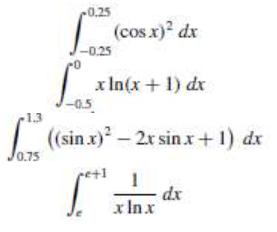
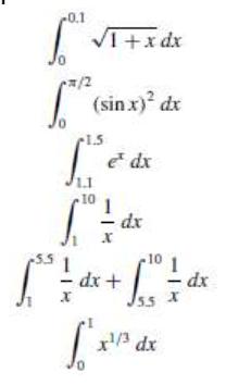
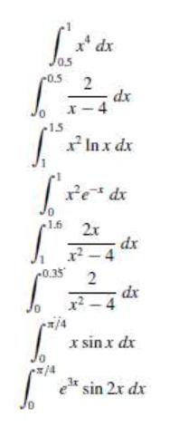
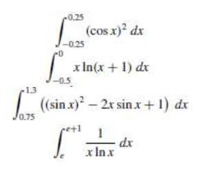
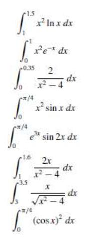
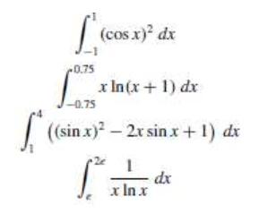
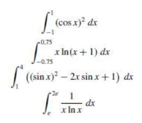
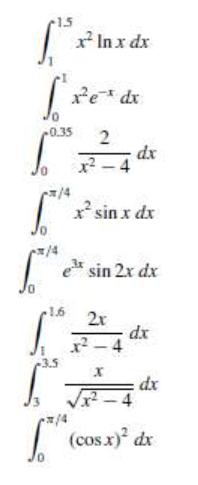
Approximate the following integrals using Gaussian quadrature with n = 2, and compare your results to the exact values of the integrals.
Approximate the following integrals using Gaussian quadrature with n = 3, and compare your results to the exact values of the integrals.
Approximate the following integrals using Gaussian quadrature with n = 4, and compare your results to the exact values of the integrals.
Approximate the following integrals using Gaussian quadrature with n = 5, and compare your results to the exact values of the integrals.
Verify the entries for the values of n = 2 and 3 in Table 4.12 on page 232 by finding the roots of the respective Legendre polynomials, and use the equations preceding this table to find the
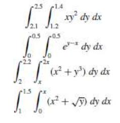
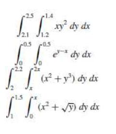
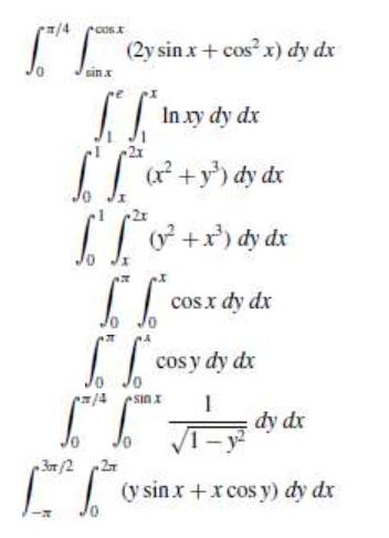
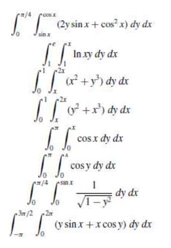
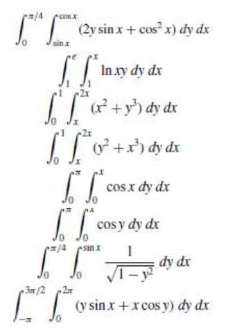
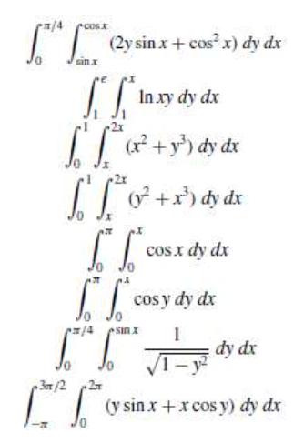
Use Algorithm 4.4 with n = m = 4 to approximate the following double integrals, and compare the results to the exact answers.
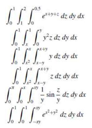
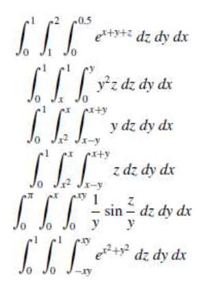
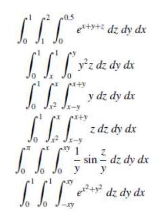
Use Algorithm 4.6 with n = m = p = 2 to approximate the following triple integrals, and compare the results to the exact answers.
Repeat Exercise 15 using n = m = p = 3.In Exercise 15
Repeat Exercise 15 using n = m = p = 4 and n = m = p = 5.In Exercise 15
Find the smallest values for n = m so that Algorithm 4.4 can be used to approximate the integrals in Exercise 1 to within 10ˆ’6 of the actual value.In Exercise 1
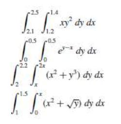
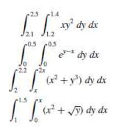
Use Algorithm 4.4 with (i) n = 4, m = 8, (ii) n = 8, m = 4, and (iii) n = m = 6 to approximate the following double integrals, and compare the results to the exact answers.
Find the smallest values for n = m so that Algorithm 4.4 can be used to approximate the integrals in Exercise 3 to within 10ˆ’6 of the actual value.In Exercise 3
Use Algorithm 4.5 with n = m = 2 to approximate the integrals in Exercise 1, and compare the results to those obtained in Exercise 1.In Exercise 1
Find the smallest values of n = m so that Algorithm 4.5 can be used to approximate the integrals in Exercise 1 to within 10ˆ’6. Do not continue beyond n = m = 5. Compare the number of functional
Use Algorithm 4.5 with (i) n = m = 3, (ii) n = 3, m = 4, (iii) n = 4, m = 3, and (iv) n = m = 4 to approximate the integrals in Exercise 3.In Exercise 3
Use Algorithm 4.5 with n = m = 5 to approximate the integrals in Exercise 3. Compare the number of functional evaluations required to the number required in Exercise 4.In Exercise 3
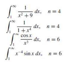
Use the transformation t = xˆ’1 and then the Composite Simpson's rule and the given values of n to approximate the following improper integrals.
The Laguerre polynomials {L0(x), L1(x) . . .} form an orthogonal set on [0,ˆž) and satisfyFor i ‰ j. The polynomial Ln(x) has n distinct zeros x1, x2, . . . , xn in [0,ˆž). LetShow that
The Laguerre polynomials L0(x) = 1, L1(x) = 1 ˆ’ x, L2(x) = x2 ˆ’ 4x + 2, and L3(x) = ˆ’x3 + 9x2 ˆ’ 18x + 6 are derived in Exercise 11 of Section 8.2. As shown in Exercise 6, these
Use Theorem 5.4 to show that each of the following initial-value problems has a unique solution, and find the solution.a. y' = y cos t, 0≤ t ≤ 1, y(0) = 1.b. y' = 2/t y + t2et, 1≤ t ≤ 2, y(1)
Show that each of the following initial-value problems has a unique solution and find the solution. Can Theorem 5.4 be applied in each case?a. y' = et−y, 0≤ t ≤ 1, y(0) = 1.b. y' = t−2(sin 2t
For each choice of f (t, y) given in parts (a)-(d): i. Does f satisfy a Lipschitz condition on D = {(t, y) | 0 ≤ t ≤ 1, −∞ < y < ∞}? ii. Can Theorem 5.6 be used to show that the
For each choice of f (t, y) given in parts (a)-(d): i. Does f satisfy a Lipschitz condition on D = {(t, y) | 0 ≤ t ≤ 1, −∞ < y < ∞}? ii. Can Theorem 5.6 be used to show that the
For the following initial-value problems, show that the given equation implicitly defines a solution. Approximate y(2) using Newton's method. a. y' = − y3 + y/((3y2 + 1)t) , 1≤ t ≤ 2, y(1) = 1;
Prove Theorem 5.3 by applying the Mean Value Theorem 1,8 to f (t, y), holding t fixed.
Show that, for any constants a and b, the set D = {(t, y) | a ≤ t ≤ b, −∞ < y < ∞} is convex.
Suppose the perturbation δ(t) is proportional to t, that is, δ(t) = δt for some constant δ. Show directly that the following initial-value problems are well-posed. a. y' = 1 − y, 0≤ t ≤ 2,
Picard's method for solving the initial-value problemy' = f (t, y), a ‰¤ t ‰¤ b, y(a) = Î±,is described as follows: Let y0(t) = Î± for each t in [a, b]. Define a sequence {yk(t)} of
To prove Theorem 5.20, part (i), show that the hypotheses imply that there exists a constant K > 0 such that |ui − vi| ≤ K|u0 − v0|, for each 1 ≤ i ≤ N, whenever {ui}Ni =1 and {vi}Ni=1
For the Adams-Bashforth and Adams-Moulton methods of order four,a. Show that if f = 0, thenF(ti , h,wi+1, . . . ,wi+1ˆ’m) = 0.b. Show that if f satisfies a Lipschitz condition with constant L,
Use the results of Exercise 32 in Section 5.4 to show that the Runge-Kutta method of order four is consistent. In Exercise 32 The Runge-Kutta method of order four can be written in the form w0 =
Consider the differential equationy' = f (t, y), a ‰¤ t ‰¤ b, y(a) = Î±.a. Show thatfor some Î¾ , where ti b. Part (a) suggests the difference methodwi+2 = 4wi+1 ˆ’ 3wi ˆ’ 2hf (ti
Given the multistep methodwi+1 = −3/2 wi + 3wi−1 - 1/2 wi−2 + 3hf (ti ,wi), for i = 2, . . . , N − 1,with starting values w0, w1, w2:a. Find the local truncation error.b. Comment on
Solve the following stiff initial-value problems using Euler's method, and compare the results with the actual solution. a. y' = −9y, 0≤ t ≤ 1, y(0) = e, with h = 0.1; actual solution y(t) =
Show that the fourth-order Runge-Kutta method, k1 = hf (ti ,wi), k2 = hf (ti + h/2,wi + k1/2), k3 = hf (ti + h/2,wi + k2/2), k4 = hf (ti + h,wi + k3), wi+1 = wi + 1/6 (k1 + 2k2 + 2k3 + k4), when
Discuss consistency, stability, and convergence for the Implicit Trapezoidal method wi+1 = wi + h/2 (f (ti+1,wi+1) + f (ti ,wi)) , for i = 0, 1, . . . , N − 1, With w0 = α applied to the
The Backward Euler one-step method is defined by wi+1 = wi + hf (ti+1,wi+1), for i = 0, . . . , N − 1. Show that Q(hλ) = 1/(1 − hλ) for the Backward Euler method.
Apply the Backward Euler method to the differential equations given in Exercise 1. Use Newton’s method to solve for wi+1.In Exercise 1a. y' = −9y, 0≤ t ≤ 1, y(0) = e, with h = 0.1; actual
Apply the Backward Euler method to the differential equations given in Exercise 2. Use Newton’s method to solve for wi+1.In Exercise 2a. y' = −5y + 6et, 0≤ t ≤ 1, y(0) = 2, with h = 0.1;
a. Show that the Implicit Trapezoidal method is A-stable. b. Show that the Backward Euler method described in Exercise 12 is A-stable.
Solve the following stiff initial-value problems using Euler's method, and compare the results with the actual solution. a. y' = −5y + 6et, 0≤ t ≤ 1, y(0) = 2, with h = 0.1; actual solution
Repeat Exercise 1 using the Runge-Kutta fourth-order method.In Exercise 1a. y' = −9y, 0≤ t ≤ 1, y(0) = e, with h = 0.1; actual solution y(t) = e1−9t .b. y' = −20(y−t2)+2t, 0≤ t ≤ 1,
Repeat Exercise 2 using the Runge-Kutta fourth-order method.In Exercise 2a. y' = −5y + 6et, 0≤ t ≤ 1, y(0) = 2, with h = 0.1; actual solution y(t) = e−5t + et .b. y' = −10y+10t+1, 0 ≤ t
Repeat Exercise 1 using the Adams fourth-order predictor-corrector method.In Exercise 1a. y' = −9y, 0≤ t ≤ 1, y(0) = e, with h = 0.1; actual solution y(t) = e1−9t .b. y' = −20(y−t2)+2t,
Repeat Exercise 2 using the Adams fourth-order predictor-corrector method.In Exercise 2a. y' = −5y + 6et, 0≤ t ≤ 1, y(0) = 2, with h = 0.1; actual solution y(t) = e−5t + et .b. y' =
Repeat Exercise 1 using the Trapezoidal Algorithm with TOL = 10−5.In Exercise 1a. y' = −9y, 0≤ t ≤ 1, y(0) = e, with h = 0.1; actual solution y(t) = e1−9t .b. y' = −20(y−t2)+2t, 0≤ t

Showing 1100 - 1200 of 3404

First
5
6
7
8
9
10
11
12
13
14
15
16
17
18
19
Last

Get In Touch

About Us
Contact Us
Career
Jobs
FAQ
Campus Ambassador

Company Info

Security
Copyrights
Privacy Policy
Terms & Condition
SolutionInn Fee
Scholarship

Services

Sitemap
Fun
Definitions
Become Tutor
Study Help Categories
Recent Questions
Expert Questions

Copyright © 2024 SolutionInn All Rights Reserved.

Get the SolutionInn - Study Help App