All Matches

Solution Library

Expert Answer

Textbooks

Search Textbook questions, tutors and Books

Oops, something went wrong!

Change your search query and then try again

Result Not Found

Books FREE
Tutors
Study Help
Ask a Question

Search
Sign In
Register

study help
mathematics
numerical analysis

Questions and Answers of Numerical Analysis

Differential equations like the one solved in Prob. 27.6 can often be simplified by linearizing their nonlinear terms. For example, a first-order Taylor series expansion can be used to linearize the
Repeat Example 27.4 but for three masses. Produce a plot like Figure to identify the principle modes of vibration. Change all the k’s to 240.
Repeat Example 27.6, but for five interior points (h = 3/6).
Use minors to expand the determinedof
Use the power method to determine the highest eigenvalue and corresponding eigenvector for Prob. 27.10.
Use the power method to determine the lowest eigenvalue and corresponding eigenvector for Prob. 27.10.
Develop a user-friendly computer program to implement the shooting method for a linear second-order ODE. Test the program by duplicating Example 27.1.
Use the program developed in Prob. 27.13 to solve Probs. 27.2 and 27.4.
Develop a user-friendly computer program to implement the finite-difference approach for solving a linear second-order ODE. Test it by duplicating Example 27.3.
Use the program developed in Prob. 27.l5 to solve Probs. 27.3 and 27.5.
Develop a user-friendly program to solve for the largest eigenvalue with the power method. Test it by duplicating Example 27.7.
Develop a user-friendly program to solve for tie smallest eigenvalue with the power method. Test it by duplicating Example 27.8.
Use the Excel Solver to directly solve (that is, without linearization) Prob. 27.6 using the finite-difference approach. Employ ∆x = 0.1 to obtain your solution.
Use MATLAB to integrate the following pair of ODEs from t = 0 to 100:dy1/dt = 0.35y1 – 1.6y1y2dy2/dt = 0.04 y1y2 – 0.15y2Where y1= 1 and y2 = 0.05 at t = 0. Develop a state- space, plot (y1
The following differential equation was used in Sec. 8.4 to analyze the vibrations of an automobile shock absorber:1.25 x 106 d2x/dt2 + 1 x 107 dx/dt + 1.5 x 109x = 0Transform this equation into a
Use IMSL to integrate(a) dx/dt = αx - bxydy/dt = -cy + dxyWhere α = 1.5, b = 0.7, c = 0.9, and d = 0.4. Employ initial conditions of x = 2 and y = 1 and integrate from t = 0 to 30.(b) dx/dt = -σx
Use finite differences to solve the boundary-value ordinary differential equationd2u/dx2 + 6du/dx – u = 2With boundary conditions u(0) = 10 and u(2) = 1. Plot the results of u versus x. Use ∆x =
Solve the nondimensionalized ODE using finite difference methods that describe the temperature distribution in a circular rod with internal heat source SOver the range 0 ≤ r ≤ 1, with the
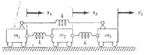
Derive the set of differential equations for a three mass-four spring system (Figure) that describes their time motion. Write the three differential equations in matrix from,[Acceleration vector] +
Consider the mass-spring system in Figure. The frequencies for the mass vibrations can be determined by solving for the eigenvalues and by applying Mx + kx = 0, which yieldsApplying the guess x =
The following nonlinear, parasitic ODE was suggested by Hornbeck (1975):dy1/dt = 5(yl – t2)If the initial condition is y1(0) = 0.08, obtain a solution from τ = 0 to 5:(a) Analytically.(b) Using
A heated rod with a uniform heat source can be modeled with the Poisson equation,d2T/dx2 = – ƒ(x)Given a heat source ƒ(x) = 25 and the boundary conditions, T(x = 0) = 40 and T(x = 10) = 200,
Repeat Prob. 27.28, but for the following heat source: ƒ(x) = 0.12x3- 2.4x2 + l2x.
Perform the first computation in Sec. 28.1, but for the case where h = 10. Use the Heun (without iteration) and the fourth-order RK method to obtain solution.
Perform the second computation in Sec. 28.1, but for the system described in Prob. 12.4.
A mass balance for a chemical in a completely mixed reactor can be written asVdc/dt = F – Qc – kVc2where V = volume (12 m3), c = concentration (g/m3), F = feed rate (175 g/min), Q = flow rate (1
If cin = cb (1 – e-0.12t), calculate the outflow concentration of a conservative substance (no reaction) for a single, completely mixed reactor as a function of time. Use Heun’s method (without
Seawater with a concentration of 8000 g/m3 is pumped into a well-mixed tank at a rate of 0.6 m3/hr. Because of faulty design work, water is evaporating from the tank at a rate of 0.025 m3/hr. The
A spherical ice cube (an ice sphere) that is 6 cm in diameter is removed from a 0°C freezer and placed on a mesh screen at room temperature Tα = 20°C. What will be the diameter of the ice cube as
The following equations define the concentrations of three reactants:dcα/dt = - 10cαcc + cbdcb/dt = 10cαcc - cbdcc/dt = - 10cαcc + cb – 2ccIf the initial conditions are cα = 50, cb = 0, and cc
Compound A diffuses through a 4-cm-long tube and reacts as it diffuses. The equation governing diffusion with reaction isDd2A/dx2 – kA = 0At one end of the tube, there is a large source of A at a
In the investigation of a homicide or accidental death, it is often important to estimate the time of death. From the experimental observations, it is known that the surface temperature of an object
The reaction A → B takes place in two reactors in series.The reactors are well mixed but are not at steady state. The unsteady-state mass balance for each tank reactor is shown below:dCAl/dt =
A nonisothermal batch reactor can be described by the following equationsdC/dt = - e(- 10/T + 273))CdT/dt = 1000e(- 10/T + 273))C – 10(T - 20)where C is the concentration of the reactant and T in
The following system is a classic example of stiff ODEs that can occur in the solution of chemical reaction kinetics:dc1/dt = – 0.013c1 – 1000c1c3dc2/dt = –2500c2c3dc3/dt = –0.013c1 –
Perform the same computation for the Lotka-Volterra system in Sec. 28.2, but use(a) Euler’s method,(b) Heun’s method (without iterating the corrector),(c) The fourth-order RK method, and(d) The
Perform the same computation for the Lorenz equations in Sec. 28.2, but use(a) Euler’s method,(b) Heun’s method (without iterating the corrector),(c) The fourth-order RK method, and(d) The MATLAB
The following equation can be used to model the deflection of a sailboat must subject to a wind force:d2y/dz2 = ƒ/2El(L - z)2where ƒ = wind force, E = modulus of elasticity, L = mast length, and l
Perform the same computation as in Prob. 28.15, but rather than using a constant wind force, employ a force that varies with height according to (recall Sec. 24.2)ƒ(z) = 200z/5 + z e-2z/30
An environmental engineer is interested in estimating the mixing that occurs between a stratified lake and an adjacent embayment (Figure). A conservative tracer is instantaneously mixed with the bay
Population-growth dynamics are important in a variety of planning studies for areas such as transportation and water resource engineering. One of the simplest models of such growth incorporates the
Although the model in Prob. 28.18 works adequately when population growth is unlimited, it breaks down when factors such as food shortages, pollution, and lack of space inhibit growth. In such cases,
Isle Royale National Park is a 210-square-mile archipelago composed of a single large island and many small islands in Lake Superior. Moose, arrived around 1900 and by 1930, their population
A cable is hanging from two supports at A and B (Figure). The cable is loaded with a distributed load whose magnitude varies with x asWhere wo = 1000 lbs/ft. The slope of the cable (dy/dx) = 0 at x =
The basic differential equation of the elastic curve for a cantilever beam (Figure) is given asEl d2y/dx2 = -P(L - x)where E = the modulus of elasticity and l = the moment of inertia. Solve for the
The basic differential equation of the elastic curve for a uniformly loaded beam (Figure) is given asEl d2y/dx2 = wLx/2 – wx2/2where E = the modulus of elasticity and l = the moment of inertia.
A pond drains through a pipe as shown in Figure. Under a number of simplifying assumptions, the following differential equation describes how depth changes with time:dh/dt = πd2/4A(h) √2g(h +
Engineers and scientists use mass-spring models to gain insight into the dynamics of structures under the influence of disturbances such as earthquakes. Figure shows such a representation for a
Perform the same computation as in the first part of Sec. 28.3, but with R = 0.025 Ω.
Solve the ODE in the first part of Sec. 8.3 from t = 0 to 0.5 using numerical techniques if q = 0.1 and i = -3.281515 at t = 0. Use an R = 50 along with the other parameters from Sec. 8.3.
For a simple RL circuit, Kirchhoff’s voltage law requires that (if Ohm’s law holds)Ldi/dt + Ri = 0where i = current, L = inductance, and R = resistance. Solve for i, if L = l, R = l.5, and i(0) =
In contrast to Prob. 28.28, real resistors may not always obey Ohm’s law. For example, the voltage drop may be nonlinear and the circuit dynamics is described by a relationship such asWhere all
Develop an eigenvalue problem for an LC network similar to the one in Figure, but with only two loops. That is, omit the i3 loop. Draw the network, illustrating how the currents oscillate in their
Perform the same computation as in Sec. 28.4 but for a l-m-long pendulum.
Section 8.4 presents a second-order differential equation that can be used to analyze the unforced oscillations of an automobile shock absorber. Given m = 1.2 x 106 g, c = l x 107 g/s, and k =l.25 x
The rate of cooling a body can be expressed asdT/dt = -k(T - Tα)where T = temperature of the body (°C), Tα = temperature of the surrounding medium (°C), and k = the proportionality constant
The rate of heat flow (conduction) between two points on a cylinder heated at one end is given bydQ/dt = λAdT/dxwhere λ = a constant, A = the cylinder’s cross-sectional area, Q = heat flow, T =
Repeat the falling parachutist problem (Example 1.2), but with the upward force due to drag as a second-order rate:Fα = -cυ2where c = 0.225 kg/m. Solve for t = 0 to 30, plot your results, and
Suppose that, after falling for 13 s, the parachutist from Examples 1.1 and 1.2 pulls the rip cord. At this point, assume that the drag coefficient is instantaneously increased to a constant value of
The following ordinary differential equation describes the motion of a damped spring-mess system (Figure):where x = displacement from the equilibrium position, t = time, m = 1 kg mass, and α = 5
A forced damped spring-mass system (Figure) has the following ordinary differential equation of motion:Where x = displacement from the equilibrium position, t = time, m = 2 kg mass, α = 5 N/(m/s)2,
The temperature distribution in a tapered conical cooling fin (Figure) is described by the following differential equation, which has been nondimensionalizedWhere u = temperature (0 ≤ u ≤ l).x =
The dynamics of a forced spring-mass-damper system can be represented by the following second-order ODE:md2x/dt2 + cdx/dt + k1x + k3x3 = P cos(ωt)where in m = 1 kg, c = 0.4 N · s/m, P = 0.5 N, and
The differential equation for the velocity of a bungee of a jumper is different depending on whether the jumper has fallen to a distance where the cord is fully extended and begins to stretch. Thus,
Use Liebmann’s method to solve for the temperature of the square heated plate in Figure, but with the upper boundary condition increased to 120°C and the left boundary decreased to 60°C. Use a
Compute the fluxes for Prob. 29.1 using the parameters from Example 29.3.
Repeat Example 29.1, but use 49 interior nodes (that is, Δx = Δy = 5 cm).
Repeat Prob. 29.3, but for the case where the lower edge is insulated.
Repeat Examples 29.1 and 29.3, but for the case where the flux at the lower edge is directed downward with a value of 1 cal/cm2 · s.
Repeat Example 29.4 for the case where both the lower left and the upper right corners are rounded in the same fashion as the lower left corner of Figure. Note that all boundary temperatures on the
With the exception of the boundary conditions, the plate in Figure has the exact same characteristics as the plate used in Examples 23.1 through 23.4. Simulate both the temperatures and fluxes for
Write equations for the darkened nodes in the grid in Figure. Note that all units are cgs. The coefficient of thermal conductivity for the plate is 0.75 cal/(s · cm · °C), the convection
Write equations for the darkened nodes in the grid in Figure. Note that all units are cgs. The convection coefficient is hc = 0.015 cal/(cm2 · C · s) and the thickness of the plate is 1.5 cm.
Apply the control volume approach to develop the equation for node (0, j) in Figure.
Derive an equation like Eq. (29.26) for the case where θ is greater than 45° for Figure.
Develop a user-friendly computer program to implement Liebmann’s method for a rectangular plate with Dirichlet boundary conditions. Design the program so that it can compute both temperature and
Employ the program from Prob. 29.12 to solve Probs. 29.1 and 29.2.
Employ the program from Prob 29.12 to solve Prob. 29.3.
Use the control-volume approach and derive the node equation for node (2, 2) in Figure and include a heat source at this point. Use the following values for the constants: Δz = 0.2.5 cm, h = 10 cm,
Calculate heat flux (W/cm2) for node (2, 2) in Figure using finite-difference approximations for the temperature gradients at this node. Calculate the flux in the horizontal direction in materials A
Repeat Example 30.1, but use the midpoint method to generate your solution.
Repeat Example 30.1, but for the case where the rod is initially at 25°C and the derivative at x = 0 is equal to 1 and at x = 10 is equal to 0. Interpret your results.
(a) Repeat Example 30.1, but for a time step of Δt = 0.05 s. Compute results to t = 0.2.(b) In addition, perform the same computation with the Heun method (without iteration of the corrector) with a
Repeat Example 30.2, but for the case where the derivative at x = 10 is equal to zero.
Repeat Example 30.3, but for Δx = 1 cm.
Repeat Example 30.5, but for the plate described in Prob. 29.1.
The advection-diffusion equation is used to compute the distribution of concentration along the length of a rectangular chemical reactor (see Sec. 32.1).∂c/∂t = D∂2c/∂x2 – U ∂c/∂x –
Develop a user-friendly computer program for the simple explicit method from Sec. 30.2. Test it by duplicating Example 30.1.
Modify the program in Prob. 30.8 so that it employs either Dirichlet or derivative boundary conditions. Test it by solving Prob. 30.2.
Develop a user-friendly computer program to implement the simple implicit scheme from Sec. 30.3. Test it by duplicating Example 30.2.
Develop a user-friendly computer program to implement the Crank-Nicolson method from Sec. 30.4. Test it by duplicating. Example 30.3
Develop a user-friendly computer program for the ADI method described in Sec. 30.5. Test it by duplicating Example 30.5.
The nondimensional form for the transient heat conduction in an insulated rod (Eq. 30.1) can be written as∂2u/∂x2 = ∂u/∂twhere nondimensional space, time, and temperature are defined asx =
The problem of transient radial heat flow in a circular rod in nondimensional form is described by∂2u/∂r2 + 1/r ∂u/∂r = ∂u/∂tBoundary conditionsu(1, l) = 1∂u/∂t(0, l) = 0Initial
Solve the following PDE:∂2u/∂x2 + b∂u/∂x = ∂u/∂tBoundary conditions u(0, l) = 0 u(1, l) = 0Initial
Determine the temperatures along a 1-m horizontal rod described by the heat conduction equation (Eq. 30.1). Assume that the right boundary is insulated and that the left boundary (x = 0) is
Repeat Example 31.1, but for T(0, t) = 75 and T(10, t) = 150 and a uniform heat source of 15.
Repeat Example 31.2, but for boundary conditions of T(0, t) = 75 and T(10, t) = 150 and a heat source of 15.
Apply the results of Prob. 31.2 to compute the temperature distribution for the entire rod using the finite-element approach.
Use Galerkin’s method to develop an element equation for a steady-state version of the advection-diffusion equation described in Prob. 30.7. Express the final result in the format of Eq. (31.26) so

Showing 600 - 700 of 3404

1
2
3
4
5
6
7
8
9
10
11
12
13
14
15
Last

Get In Touch

About Us
Contact Us
Career
Jobs
FAQ
Campus Ambassador

Company Info

Security
Copyrights
Privacy Policy
Terms & Condition
SolutionInn Fee
Scholarship

Services

Sitemap
Fun
Definitions
Become Tutor
Study Help Categories
Recent Questions
Expert Questions

Copyright © 2024 SolutionInn All Rights Reserved.

Get the SolutionInn - Study Help App