All Matches

Solution Library

Expert Answer

Textbooks

Search Textbook questions, tutors and Books

Oops, something went wrong!

Change your search query and then try again

Result Not Found

Books FREE
Tutors
Study Help
Ask a Question

Search
Sign In
Register

study help
mathematics
numerical analysis

Questions and Answers of Numerical Analysis

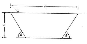
As an agricultural engineer, you must design a trapezoidal open channel to carry irrigation water (Figure). Determine the optimal dimensions to minimize the wetted perimeter for a cross-sectional
Find the optimal dimensions for a heated cylindrical tank designed to hold 10 m3 of fluid. The ends and sides cost $200/m2 and $100/m2, respectively. In addition, a coating is applied to the entire
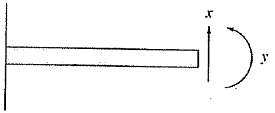
A finite-element model of a cantilever beam subject to loading and moments (Figure) is given by optimizing ?(x, y) = 5x2 ? 5xy + 2.5y2 ? x ? 1.5y Where x = end displacement and y = end moment. Find
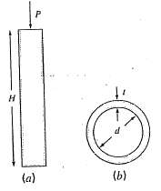
Suppose that you are asked to design a column to support a compressive load P as shown in Figure. The column has a cross-section shaped as a thin-walled pipe as shown in Figure. The design variables
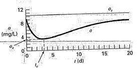
The Streeter-Phelps model can be used to compute the dissolved oxygen concentration in a river below a point discharge of sewage (Figure), o = os?? kdLo/kd + ks ? ka (e?kat?? e?(kd + ks)t) ?
The two-dimensional distribution of pollutant concentration in a channel can be described byc(x, y) = 7.7 + 0.15x + 0.22y – 0.05x2–0.016y2 – 0.007xyDetermine the exact location of the peak
The flow Q [m3/s] in an open channel can be predicted with the Manning equation (recall Sec. 8.2)Q = 1/n AcR2/3 S1/2Where n = Manning roughness coefficient (a dimensionless number used to
A cylindrical beam carries a compression load P = 3000 kN. To prevent the beam from buckling, this load must be less than a critical load,Pc = π2El/L2Where E = Young’s modulus = 200 x 109 N/m2, I
The Splash River has a flow rate of 2 x 106 m3/d, of which up to 70% can be diverted into two channels where it flows through Splish County. These channels are used for transportation, irrigation,
Determine the beam cross-sectional areas that result in the minimum weight for the truss we studied in Sec. 12.2 (Figure). The critical buckling and maximum tensile strengths of compression and
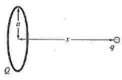
A total charge Q is uniformly distributed around a ring-shaped conductor with radius ?. A charge q is located at a distance x from the center of the ring (Figure). The force exerted on the charge by
A system consists of two power plants that must deliver loads over a transmission network. The costs of generating power at plants 1 and 2 are given byF1 = 2p1 + 2F2 = 10p2Where p1 and p2 = power
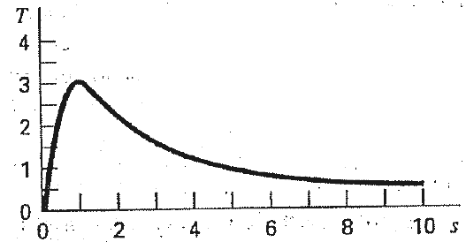
The torque transmitted to an induction motor is a function of the slip between the rotation of the stator field and the rotor speed s where slip is defined as s = n ? nR/n Where n = revolutions per
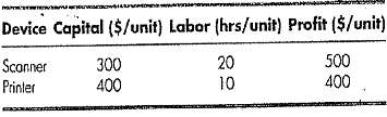
(a) A computer equipment manufacturer produces scanners and printers. The resources needed for producing these devices and the corresponding profits are If there are $127,000 worth of capital and
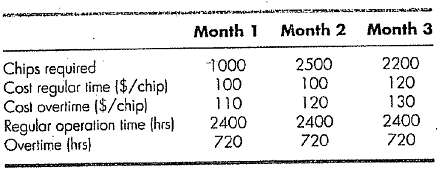
A manufacturer provides specialized microchips. During the next 3 months its sales, costs, and available time are There are no chips in stock at the beginning of the first month. It takes 1.5 hrs
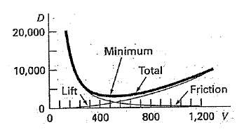
The total drag on an airfoil can be estimated by D = 0.01?V2 + 0.95/? (W/V)2 Friction ? ? ? ? ? ? ? ? ? ? ? ?lift Where D = drag, ? = ratio of air density between the flight altitude and sea level, W
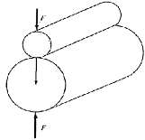
Roller bearings are subject to fatigue failure caused by large contacts loads F (Figure). The problem of finding the location of the maximum stress along the x axis can be shown to be equivalent to
An aerospace company is developing a new fuel additive for commercial airliners. The additive is composed of three ingredients: X, Y, and Z. For peak performance, the total amount of additive must be
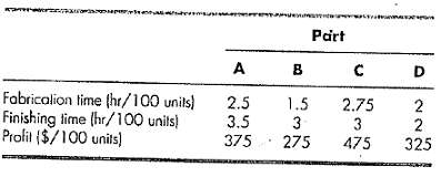
A manufacturing firm produces five types of automobile parts. Each is first fabricated and then finished. The required worker hours and profit for each part are The capacities of the fabrication
Given the data8.8 9.59.8 9.410.09.410.19.211.3 9.410.010.47.910.4 9.89.8 9.58.9 8.810.610.1 9.59.610.2 8.9Determine(a) The mean,(b) The standard deviation,(c) The variance,(d) The coefficient of
Construct a histogram from the data from Prob. 17.1. Use a range from 7.5 to 11.5 with intervals of 0.5.
Given the data28.6526.5526.6527.6527.3528.3526.8528.6529.6527.8527.0528.2528.8526.7527.6528.4528.6528.4531.6526.3527.7529.2527.6528.6527.6528.5527.6527.25Determine(a) The mean,(b) The standard
Use least-squares regression to fit a straight toAlong with the slope and intercept, compute the standard error of the estimate and the correlation coefficient. Plot the data and the regression line.
Use least-squares regression to fit a straight toAlong with the slope and the intercept, compute the standard error of the estimate and the correlation coefficient. Plot the data and the regression
Using the same approach as was employed to derive Eqs. (17.15) and (17.16), derive the least-squares fit of the following model:y = α1 x + eThat is, determine the slope that results in the
Use least-squares regression to fit a straight to(a) Along with the slope and intercept, compute the standard error of the estimate and the correlation coefficient. Plot the data and the straight
Fit the following data with(a) A saturation-growth-rate model,(b) A power equation, and(c) A parabola. In each case, Plot the data and theequation.
Fit the following data with the power model (y = αx-b). Use the resulting power equation to predict y at x = 9:
Fit an exponential model toPlot the data and the equation on both standard and semi-logarithmic graphpaper.
Rather than using the base-e exponential model (Eq. 17.22), a common alternative is to use a base-10 model,y = α5 10βsxWhen used for curve fitting, this equation yields identical results to the
Beyond the examples in Figure, there are other models that can be linearized using transformations. For example,y = α4xeβ4xLinearize this model and use it to estimate α4 and β4 based on the
An investigator has reported the data tabulated below for an experiment to determine the growth rate of bacteria k (per d), as a function of oxygen concentration c (mg/L). It is known that such data
Given the dataUse least-squares regression to fit(a) A straight line,(b) A power equation,(c) A saturation-growth-rate equation, and(d) A parabola. Plot the data along with all the curves. Is any one
Fit a cubic equation to the following data:Along with the coefficients, determine r2 andsy/x.
Use multiple linear regression to fitCompute the coefficients, the standard error of the estimate, and the correlationcoefficient.
Use multiple linear regression to fitCompute the coefficients, the standard error of the estimate, and the correlationcoefficient.
Use nonlinear regression to fit a parabola to the followingdata:
Use nonlinear regression to fit a saturation-growth-rate equation to the data in Prob. 17. 14.
Recompute the regression fits from Probs.(a) 17.4, and(b) 17.15, using the matrix approach. Estimate the standard errors and develop 90% confidence intervals for the coefficients.
Develop, debug, and test a program in either a high-level language or macro language of your choice to implement linear regression. Among other things:(a) Include statements to document the code,
A material is tested for cyclic fatigue failure whereby a stress, in MPa, is applied to the material and the number of cycles needed to cause failure is measured. The results are in the table below.
The following data shows the relationship between the viscosity of SAE 70 oil and temperature. After taking the log of the data, use linear regression to find the equation of the line that best fits
The data below represents the bacterial growth in a liquid culture over a number of days.Find a best-fit equation to the data trend. Try several possibilities-linear, parabolic, and exponential. Use
The concentration of E. coli bacteria in a swimming area is monitored after a storm:The time is measured in hours following the end of the storm and the unit CFU is a "colony forming unit" Use this
An object is suspended in a wind tunnel and the force measured for various levels of wind velocity. The results are tabulated below. Use least-squares regression to fit a straight line to this
Fit a power model to the data from Prob. 17.26, but use natural logarithms to perform the transformations.
Using the same approach as was employed to derive Eqs. (17.15) and (17.16), derive the least-squares fit of the following model:y = α1x + α2x2 + eThat is, determine the coefficients that results in
In Prob. 17.12 we used transformations to linearize and fit the following model:y = α4xeβ4xUse nonlinear regression to estimate α4 and β4 based on the following data. Develop a Plot of your fit
Estimate the common logarithm of 10 using-linear interpolation.(a) Interpolate between log 8 = 0.903900 and log 12 = 1.0791812.(b) Interpolate between log 9 = 0.9542425 and log 11 = 1.0413927. For
Fit a second-order Newton’s interpolating polynomial to estimate log 10 using the data from Prob. 18.1 at x = 8, 9, and 11. Compute the true percent relative error.
Fit a third-order Newton’s interpolating polynomial to estimate log 10 using the data from Prob. 18.1.
Given the data(a) Calculate ƒ(2.8) using Newton’s interpolating polynomials of order 1 through 3. Choose the sequence of the points for your estimates to attain the best possible accuracy.(b)
Given the data Calculate ƒ(4) using Newton’s interpolating polynomials of order 1 through 4. Choose your base points to attain good accuracy. What do your results indicate regarding the order of
Repeat Probs. 18.1 through 18.3 using the Lagrange polynomial.
Repeat Prob. 18.5 using Lagrange polynomials of order 1 through 3.
Employ inverse interpolation using a cubic interpolating polynomial and bisection to determine the value of x that corresponds to Æ’(x) = 0.23 for the following tabulateddata:
Employ inverse interpolation to determine the value of x that corresponds to Æ’(x) = 0.85 for the following tabulated data:Note that the values in the table ware generated with the
Develop quadratic splines for the first 5 data points in Prob. 18.4 and predict ƒ(3.4) and ƒ(2.2).
Develop cubic splines for the data in Prob. 18.5 and(a) Predict ƒ(4) and ƒ(2.5) and(b) Verify that ƒ2(3) and ƒ3(3) = 19.
Determine the coefficients of the parabola that passes through the last three points in Prob. 18.4.
Determine the coefficients of the cubic equation that passes through the first four points in Prob. 18.5.
Develop, debug, and test a program in either a high-level language or macro language of your choice to implement Newton’s interpolating polynomial based on Figure.
Test the program you developed in Prob. 18.14 by duplicating the computation from Example 18.5.
Use the program you developed in Prob. 18.14 to solve Probs. 18.1 through 18.3.
Use the program you developed in Prob. 18.14 to solve Probs. 18.4 and 18.5. In Problem 18.4, utilized all data to develop first- through fifth-order polynomials. For both problems, plot the estimated
Develop, debug, and test a program in either a high-level language or macro language of your choice to implement Lagrange interpolation. Base it on the pseudocode from Figure. Test it by duplicating
A useful application of Lagrange interpolation is called a table look-up. As the name implies, this involves “looking-up” an intermediate value from a table. To develop such an algorithm, the
Develop, debug, and test a program in either a high-level language or macro language of your choice to implement cubic spline interpolation based on Figure. Test the program by duplicating Example
Use the software developed in Prob. 18.20 to fit cubic splines through the data in Probs. 18.4 and 18.5. For both cases, predict ƒ(2.25).
Use the portion of the given steam table for superheated H2O at 200 MPa to(a) Find the corresponding entropy s for a specific volume v of 0.108 m3/kg with linear interpolation,(b) Find the same
The pH in a reactor varies sinusoidally over the course of a day. Use least-squares regression to fit Eq. (19.11) to the following data. Use your fit to determine the mean, amplitude, and time of
The solar radiation for Tucson, Arizona, has been tabulated asAssuming each month is 30 days long, fit a sinusoid to this data. Use the resulting equation to predict the radiation inmid-August.
The average values of a function can be determined byUse this relationship to verify the results of Eq.(19.13).
Use a continuous Fourier series to approximate the sawtooth wave in Figure. Plot the first three terms along with thesummation.
Use a continuous Fourier series to approximate the wave from in Figure. Plot the first three terms along with thesummation.
Construct amplitude and phase line spectra for Prob. 19.4.
Construct amplitude and phase line spectra for Prob. 19.5.
A half-wave rectifier can be characterized bywhere C1 is the amplitude of the wave. Plot the first four terms along with thesummation.
Construct amplitude and phase line spectra for Prob. 19.8.
Develop a user-friendly program for the DFT based on the algorithm from Figure. Test it by duplicatingFigure.
Use the program from Prob. 19.10 to compute a DFT for the triangular wave from Prob. 19.8. Sample the wave from t = 0 to 4T. Use 32, 64, and 128 sample points. Time each run and plot execution versus
Develop a user-friendly program for the FFT based on the algorithm from Figure. Test it by duplicating Figure.
Repeat Prob. 19.11 using the software you developed in Prob. 19.12.
An object is suspended in a wind tunnel and the force measured for various levels of wind velocity. The results are tabulated below. Use Excel’s Trendline command to fit a power equation to this
Use the Excel Data Analysis Toolpack to develop a regression polynomial to the following data for the dissolved oxygen concentration of fresh water versus temperature at sea level. Determine the
Use the Excel Data Analysis Toolpack to fit a straight line to the following data. Determine the 90% confidence interval for the intercept. If it encompasses zero, redo the regression, but with the
(a) Use MATLAB to fit a cubic spline to the following data:Determine the value of y at x = 1.5.(b) Repeat (a), but with zero first derivatives at the end knots. Note that the MATLAB help facility
Use MATLAB to generate 64 points from the functionƒ(t) = cos(10t) + sin(3t)from t = 0 to 2π. Add a random component to the signal with the function randn. Take an FFT of these values and plot the
In a fashion similar to Sec. 19.8.2, use MATLAB to fit the data from Prob. 19.15 using(a) Linear interpolation,(b) A third-order regression polynomial, and(c) A spline. Use each approach to predict
Runge’s function is written asƒ(x) = 1/1 + 25x2Generate 9 equidistantly spaced values of this function over the interval: [-1, 1]. Fit this data with(a) An eighth-order polynomial,(b) A linear
Repeat Prob. 19.15, but use the IMSL routine, RCURV.
A dye is injected into the circulating blood volume to measure a patient’s cardiac output, which is the volume flow rate of blood out of the left ventricle of the heart. In other words, cardiac
In electric circuits, it is common to see current behavior in the form of a square ware as shown in Figure. Solving for the Fourier series fromWe get the Fourier seriesLet A0 = 1 and T = 0.25 s. Plot
Develop a plot of the following data with(a) Sixth-order interpolating polynomial,(b) A cubic spline, and(c) A cubic spline with zero end derivatives.In each case, compare your plot with the
Perform the same computation as in Sec. 20.1, but use linear regression and transformations to fit the data with a power equation. Assess the result.
You perform experiments and determine the following values of heat capacity c at various temperatures T for a gas:Use regression to determine a model to predict c as a function ofT.
The saturation concentration of dissolved oxygen in water as a function of temperature and chloride concentration is listed Table P20.3. Use interpolation to estimate the dissolved oxygen level for
For the data in Table P20.3, use polynomial regression to derive a third-order predictive equation for dissolved oxygen concentration as a function of temperature for the case where chloride
Use multiple linear regression to derive a predictive equation for dissolved oxygen concentration as a function of temperature and chloride based on the data from Table P20.3. Use the equation to
As compared to the models from Probs. 20.4 and 20.5, a somewhat more sophisticated model that accounts for the effect of both temperature and chloride on dissolved oxygen saturation can be

Showing 400 - 500 of 3404

1
2
3
4
5
6
7
8
9
10
11
12
13
14
15
Last

Get In Touch

About Us
Contact Us
Career
Jobs
FAQ
Campus Ambassador

Company Info

Security
Copyrights
Privacy Policy
Terms & Condition
SolutionInn Fee
Scholarship

Services

Sitemap
Fun
Definitions
Become Tutor
Study Help Categories
Recent Questions
Expert Questions

Copyright © 2024 SolutionInn All Rights Reserved.

Get the SolutionInn - Study Help App