New Semester Started Get 50% OFF Study Help! --h --m --s Claim Now

Question Answers

Textbooks

Find textbooks, questions and answers

Oops, something went wrong!

Change your search query and then try again

Result Not Found

Books FREE
Study Help
Tutors
AI Study Planner NEW
Sell Books

Search
Sign In
Register

study help
mathematics
statistics

Elementary Statistics 8th Edition Neil A. Weiss - Solutions

Suppose that a random sample of size 1 is to be taken from a finite population of size N. a. How many possible samples are there? b. Identify the relationship between the possible sample means and the possible observations of the variable under consideration. c. What is the difference between
Population data: 1, 2, 3.a. Find the mean, μ, of the variable.b. For each of the possible sample sizes, construct a table similar to Table 7.2 on page 281 and draw a dotplot for the sampling distribution of the sample mean similar to Fig. 7.1 on page 281.c. Construct a graph similar to Fig. 7.3
In this section, we stated that, when the sample size is small relative to the population size, there is little difference between sampling with and without replacement. Explain in your own words why that statement is true.
Refer to Exercise 7.3 on page 283. Population data: 1, 2, 3. a. Use your answers from Exercise 7.3(b) to determine the mean, μx-bar, of the variable x-bar for each of the possible sample sizes. b. For each of the possible sample sizes, determine the mean, μx-bar, of the variable x-bar, using only
Refer to Exercise 7.4 on page 283.Population data: 2, 5, 8.a. Use your answers from Exercise 7.4(b) to determine the mean, μx-bar of the variable x-bar for each of the possible sample sizes.b. For each of the possible sample sizes, determine the mean, μx-bar of the variable x-bar, using only your
Refer to Exercise 7.5 on page 283.Population data: 1, 2, 3, 4.a. Use your answers from Exercise 7.5(b) to determine the mean, μx-bar of the variable x-bar for each of the possible sample sizes.b. For each of the possible sample sizes, determine the mean, μx-bar of the variable x-bar, using only
Refer to Exercise 7.6 on page 283.Population data: 3, 4, 7, 8.a. Use your answers from Exercise 7.6(b) to determine the mean, μx-bar, of the variable x-bar, for each of the possible sample sizes.b. For each of the possible sample sizes, determine the mean, μx-bar, of the variable x-bar, using
Refer to Exercise 7.7 on page 284.Population data: 1, 2, 3, 4, 5.a. Use your answers from Exercise 7.7(b) to determine the mean, μx-bar, of the variable x-bar, for each of the possible sample sizes.b. For each of the possible sample sizes, determine the mean, μx-bar, of the variable x-bar, using
Refer to Exercise 7.8 on page 284.Population data: 2, 3, 5, 7, 8.a. Use your answers from Exercise 7.8(b) to determine the mean, μx-bar, of the variable x-bar for each of the possible sample sizes.b. For each of the possible sample sizes, determine the mean, μx-bar, of the variable x-bar using
Refer to Exercise 7.9 on page 284.Population data: 1, 2, 3, 4, 5, 6.a. Use your answers from Exercise 7.9(b) to determine the mean, μx-bar, of the variable x-bar for each of the possible sample sizes.b. For each of the possible sample sizes, determine the mean, μx-bar, of the variable x-bar using
Population data: 2, 5, 8.a. Find the mean, μ, of the variable.b. For each of the possible sample sizes, construct a table similar to Table 7.2 on page 281 and draw a dotplot for the sampling distribution of the sample mean similar to Fig. 7.1 on page 281.c. Construct a graph similar to Fig. 7.3
Refer to Exercise 7.10 on page 284.Population data: 2, 3, 5, 5, 7, 8.a. Use your answers from Exercise 7.10(b) to determine the mean, μx-bar, of the variable x-bar for each of the possible sample sizes.b. For each of the possible sample sizes, determine the mean, μx-bar, of the variable x-bar,
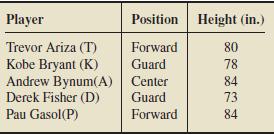
The winner of the 2008–2009 National Basketball Association (NBA) championship was the Los Angeles Lakers. One starting lineup for that team is shown in the following table.a. Determine the population mean height, μ, of the five players.b. Consider samples of size 2 without replacement. Use your
Repeat parts (b) and (c) of Exercise 7.41 for samples of size 1. For part (b), use your answer to Exercise 7.12(b).b. Consider samples of size 2 without replacement. Use your answer to Exercise 7.11(b) on page 284 and Definition 3.11 on page 128 to find the mean, μx-bar, of the variable x-bar.c.
Repeat parts (b) and (c) of Exercise 7.41 for samples of size 3. For part (b), use your answer to Exercise 7.13(b).b. Consider samples of size 2 without replacement. Use your answer to Exercise 7.11(b) on page 284 and Definition 3.11 on page 128 to find the mean, Î¼x-bar, of the
Repeat parts (b) and (c) of Exercise 7.41 for samples of size 4. For part (b), use your answer to Exercise 7.14(b).b. Consider samples of size 2 without replacement. Use your answer to Exercise 7.11(b) on page 284 and Definition 3.11 on page 128 to find the mean, Î¼x-bar, of the
Repeat parts (b) and (c) of Exercise 7.41 for samples of size 5. For part (b), use your answer to Exercise 7.15(b).b. Consider samples of size 2 without replacement. Use your answer to Exercise 7.11(b) on page 284 and Definition 3.11 on page 128 to find the mean, Î¼x-bar, of the
According to the Bureau of Labor Statistics publication News, self-employed persons with home-based businesses work a mean of 25.4 hours per week at home. Assume a standard deviation of 10 hours. a. Identify the population and variable. b. For samples of size 100, find the mean and standard
The paper "Are Babies Normal?" by T. Clemons and M. Pagano (The American Statistician, Vol. 53, No. 4, pp. 298-302) focused on birth weights of babies. According to the article, the mean birth weight is 3369 grams (7 pounds, 6.5 ounces) with a standard deviation of 581 grams. a. Identify the
In the article "Age at Menopause in Puebla, Mexico" (Human Biology, Vol. 75, No. 2, pp. 205-206), authors L. Sievert and S. Hautaniemi compared the age of menopause for different populations. Menopause, the last menstrual period, is a universal phenomenon among females. According to the article,
According to the U.S. Census Bureau publication Manufactured Housing Statistics, the mean price of new mobile homes is $65,100. Assume a standard deviation of $7200. Let x-bar denote the mean price of a sample of new mobile homes. a. For samples of size 50, find the mean and standard deviation of
Population data: 1, 2, 3, 4.a. Find the mean, μ, of the variable.b. For each of the possible sample sizes, construct a table similar to Table 7.2 on page 281 and draw a dotplot for the sampling distribution of the sample mean similar to Fig. 7.1 on page 281.c. Construct a graph similar to Fig. 7.3
S. Parker et al. analyzed the labor supply of self-employed individuals in the article "Wage Uncertainty and the Labour Supply of Self-Employed Workers" (The Economic Journal, Vol. 118, No. 502, pp. C190-C207). According to the article, the mean age of a self-employed individual is 46.6 years with
According to The Earth: Structure, Composition and Evolution (The Open University, S237), for earthquakes with a magnitude of 7.5 or greater on the Richter scale, the time between successive earthquakes has a mean of 437 days and a standard deviation of 399 days. Suppose that you observe a sample
The U.S. Department of Health and Human Services publishes information on AIDS in Morbidity and Mortality Weekly Report. During one year, the number of provisional cases of AIDS for each of the 50 states are as presented on the WeissStats CD. Use the technology of your choice to solve the following
Each year, thousands of high school students bound for college take the Scholastic Assessment Test (SAT).This test measures the verbal and mathematical abilities of prospective college students. Student scores are reported on a scale that ranges from a low of 200 to a high of 800. Summary results
A statistic is said to be an unbiased estimator of a parameter if the mean of all its possible values equals the parameter; otherwise, it is said to be a biased estimator. An unbiased estimator yields, on average, the correct value of the parameter, whereas a biased estimator does not. a. Is the
Suppose that a simple random sample is taken without replacement from a finite population of size N. a. Show mathematically that Equations (7.1) and (7.2) are identical for samples of size 1. b. Explain in words why part (a) is true. c. Without doing any computations, determine σ. x for samples of
In Example 7.5, we used the definition of the standard deviation of a variable (Definition 3.12 on page 130) to obtain the standard deviation of the heights of the five starting players on a men's basketball team and also the standard deviation of x-bar for samples of sizes 1, 2, 3, 4, and 5. The
Consider simple random samples of size n without replacement from a population of size N.a. Show that if n ‰¤ 0.05N, thenb. Use part (a) to explain why there is little difference in the values provided by Equations (7.1) and (7.2) when the sample size is small relative to the population
This exercise can be done individually or, better yet, as a class project.a. Use a random-number table or random-number generator to obtain a sample (with replacement) of four digits between 0 and 9. Do so a total of 50 times and compute the mean of each sample.b. Theoretically, what are the mean
Population data: 3, 4, 7, 8.a. Find the mean, μ, of the variable.b. For each of the possible sample sizes, construct a table similar to Table 7.2 on page 281 and draw a dotplot for the sampling distribution of the sample mean similar to Fig. 7.1 on page 281.c. Construct a graph similar to Fig. 7.3
For humans, gestation periods are normally distributed with a mean of 266 days and a standard deviation of 16 days. Suppose that you observe the gestation periods for a sample of nine humans.a. Theoretically, what are the mean and standard deviation of all possible sample means?b. Use the
Desert Samaritan Hospital in Mesa, Arizona, keeps records of emergency room traffic. Those records reveal that the times between arriving patients have a special type of reverse-J-shaped distribution called an exponential distribution. They also indicate that the mean time between arriving patients
Identify the two different cases considered in discussing the sampling distribution of the sample mean. Why do we consider those two different cases separately?
A variable of a population has a mean of μ = 100 and a standard deviation of σ = 28. a. Identify the sampling distribution of the sample mean for samples of size 49. b. In answering part (a), what assumptions did you make about the distribution of the variable? c. Can you answer part (a) if the
A variable of a population has a mean of μ = 35 and a standard deviation of σ = 42. a. If the variable is normally distributed, identify the sampling distribution of the sample mean for samples of size 9. b. Can you answer part (a) if the distribution of the variable under consideration is
A variable of a population is normally distributed with mean μ and standard deviation σ. a. Identify the distribution of x-bar. b. Does your answer to part (a) depend on the sample size? Explain your answer. c. Identify the mean and the standard deviation of x-bar. d. Does your answer to part (c)
A variable of a population has mean μ and standard deviation σ. For a large sample size n, answer the following questions.a. Identify the distribution of x-bar.b. Does your answer to part (a) depend on n being large? Explain your answer.c. Identify the mean and the standard deviation of x-bar.d.
Refer to Fig. 7.6 on page 295.a. Why are the four graphs in Fig. 7.6(a) all centered at the same place?b. Why does the spread of the graphs diminish with increasing sample size? How does this result affect the sampling error when you estimate a population mean, μ, by a sample mean, x-bar?c. Why
According to the central limit theorem, for a relatively large sample size, the variable x-bar is approximately normally distributed. a. What rule of thumb is used for deciding whether the sample size is relatively large? b. Roughly speaking, what property of the distribution of the variable under
In 1905, R. Pearl published the article "Biometrical Studies on Man. I. Variation and Correlation in Brain Weight" (Biometrika, Vol. 4, pp. 13-104). According to the study, brain weights of Swedish men are normally distributed with a mean of 1.40 kg and a standard deviation of 0.11 kg.a. Determine
Population data: 1, 2, 3, 4, 5.a. Find the mean, μ, of the variable.b. For each of the possible sample sizes, construct a table similar to Table 7.2 on page 281 and draw a dotplot for the sampling distribution of the sample mean similar to Fig. 7.1 on page 281.c. Construct a graph similar to Fig.
As reported by Runner's World magazine, the times of the finishers in the New York City 10-km run are normally distributed with a mean of 61 minutes and a standard deviation of 9 minutes. Do the following for the variable "finishing time" of finishers in the New York City 10-km run.a. Find the
Data on salaries in the public school system are published annually in National Survey of Salaries and Wages in Public Schools by the Education Research Service. The mean annual salary of (public) classroom teachers is $49.0 thousand. Assume a standard deviation of $9.2 thousand. Do the following
B. Ciochetti et al. studied mortgage loans in the article "A Proportional Hazards Model of Commercial Mortgage Default with Originator Bias" (Journal of Real Estate and Economics, Vol. 27, No. 1, pp. 5-23). According to the article, the loan amounts of loans originated by a large insurancecompany
In the article "A Multifactorial Intervention Program Reduces the Duration of Delirium, Length of Hospitalization, and Mortality in Delirious Patients" (Journal of the American Geriatrics Society, Vol. 53, No. 4, pp. 622-628), M. Lundstrom et al. investigated whether education programs for nurses
In the article "Job Mobility and Wage Growth" (Monthly Labor Review, Vol. 128, No. 2, pp. 33-39), A. Light examined data on employment and answered questions regarding why workers separate from their employers. According to the article, the standard deviation of the length of time that women with
An air conditioning contractor is preparing to offer service contracts on the brand of compressor used in all of the units her company installs. Before she can work out the details, she must estimate how long those compressors last, on average. The contractor anticipated this need and has kept
The R. R. Bowker Company collects information on the retail prices of books and publishes its findings in The Bowker Annual Library and Book Trade Almanac. In 2005, the mean retail price of all history books was $78.01. Assume that the standard deviation of this year's retail prices of all history
Calcium is the most abundant mineral in the human body and has several important functions. Most body calcium is stored in the bones and teeth, where it functions to support their structure. Recommendations for calcium are provided in Dietary Reference Intakes, developed by the Institute of
Dementia is the loss of the intellectual and social abilities severe enough to interfere with judgment, behavior, and daily functioning. Alzheimer's disease is the most common type of dementia. In the article "Living with Early Onset Dementia: Exploring the Experience and Developing Evidence-Based
A study by M. Chen et al. titled "Heat Stress Evaluation and Worker Fatigue in a Steel Plant" (American Industrial Hygiene Association, Vol. 64, pp. 352-359) assessed fatigue in steel-plant workers due to heat stress. If the mean post-work heart rate for casting workers equals the normal resting
Population data: 2, 3, 5, 7, 8.a. Find the mean, μ, of the variable.b. For each of the possible sample sizes, construct a table similar to Table 7.2 on page 281 and draw a dotplot for the sampling distribution of the sample mean similar to Fig. 7.1 on page 281.c. Construct a graph similar to Fig.
A variable of a population is normally distributed with mean μ and standard deviation σ. For samples of size n, fill in the blanks. Justify your answers. a. 68.26% of all possible samples have means that lie within of the population mean, μ. b. 95.44% of all possible samples have means that lie
A variable of a population has mean μ and standard deviation σ. For a large sample size n, fill in the blanks. Justify your answers. a. Approximately % of all possible samples have means within σ/√n of the population mean, μ. b. Approximately % of all possible samples have means within
A brand of water-softener salt comes in packages marked "net weight 40 lb." The company that packages the salt claims that the bags contain an average of 40 lb of salt and that the standard deviation of the weights is 1.5 lb. Assume that the weights are normally distributed.a. Obtain the
In Example 7.9 on page 294, we conducted a simulation to check the plausibility of the central limit theorem. The variable under consideration there is household size, and the population consists of all U.S. households. A frequency distribution for household size of U.S. households is presented in
For humans, gestation periods are normally distributed with a mean of 266 days and a standard deviation of 16 days. Suppose that you observe the gestation periods for a sample of nine humans.a. Use the technology of your choice to simulate 2000 samples of nine human gestation periods each.b. Find
A variable is said to have an exponential distribution or to be exponentially distributed if its distribution has the shape of an exponential curve, that is, a curve of the form y = e−x/μ/μ for x > 0, where μ is the mean of the variable. The standard deviation of such a variable also equals
Population data: 1, 2, 3, 4, 5, 6.a. Find the mean, μ, of the variable.b. For each of the possible sample sizes, construct a table similar to Table 7.2 on page 281 and draw a dotplot for the sampling distribution of the sample mean similar to Fig. 7.1 on page 281.c. Construct a graph similar to
In the Southern Ocean food web, the krill species Euphausia superba is the most important prey species for many marine predators, from seabirds to the largest whales. Body lengths of the species are normally distributed with a mean of 40 mm and a standard deviation of 12 mm. a. Sketch the normal
Refer to Problem 10. In problem In the Southern Ocean food web, the krill species Euphausia superba is the most important prey species for many marine predators, from seabirds to the largest whales. Body lengths of the species are normally distributed with a mean of 40 mm and a standard deviation
The following graph shows the curve for a normally distributed variable. Superimposed are the curves for the sampling distributions of the sample mean for two different sample sizes.a. Explain why all three curves are centered at the same place. b. Which curve corresponds to the larger sample size?
In the article "Drinking Glucose Improves Listening Span in Students Who Miss Breakfast" (Educational Research, Vol. 43, No. 2, pp. 201-207), authors N. Morris and P. Sarll explored the relationship between students who skip breakfast and their performance on a number of cognitive tasks. According
The American Council of Life Insurers provides information about life insurance in force per covered family in the Life Insurers Fact Book. Assume that the standard deviation of life insurance in force is $50,900. a. Determine the probability that the sampling error made in estimating the
A paint manufacturer in Pittsburgh claims that his paint will last an average of 5 years. Assuming that paint life is normally distributed and has a standard deviation of 0.5 year, answer the following questions:a. Suppose that you paint one house with the paint and that the paint lasts 4.5 years.
In the paper "Cloudiness: Note on a Novel Case of Frequency" (Proceedings of the Royal Society of London, Vol. 62, pp. 287-290), K. Pearson examined data on daily degree of cloudiness, on a scale of 0 to 10, at Breslau (Wroclaw), Poland, during the decade 1876-1885. A frequency distribution of the
The Graduate Record Examination (GRE) is a standardized test that students usually take before entering graduate school. According to the document Interpreting Your GRE Scores, a publication of the Educational Testing Service, the scores on the quantitative portion of the GRE are (approximately)
A variable is said to be uniformly distributed or to have a uniform distribution with parameters a and b if its distribution has the shape of the horizontal line segment y = 1/(b − a), for a < x < b. The mean and standard deviation of such a variable are (a + b)/2 and (b − a)/√ 12,
a. What percentage of the waybills constituted the sample? b. What percentage error was made by using the sample to estimate the total revenue due C&O? c. At the time of the study, the cost of a census was approximately $5000, whereas the cost for the sample estimate was only $1000. Knowing this
What is the sampling distribution of a statistic? Why is it important?
Relative to the population mean, what happens to the possible sample means for samples of the same size as the sample size increases? Explain the relevance of this property in estimating a population mean by a sample mean.
In 2005, the Internal Revenue Service (IRS) sampled 292,966 tax returns to obtain estimates of various parameters. Data were published in Statistics of Income, Individual Income Tax Returns. According to that document, the mean income tax per return for the returns sampled was $10,319. a. Explain
The following table gives the monthly salaries (in $1000s) of the six officers of a company.a. Calculate the population mean monthly salary, Î¼. There are 15 possible samples of size 4 from the population of six officers. They are listed in the first column of the following table. b.
Comerica Bank publishes information on new car prices in Comerica Auto Affordability Index. In the year 2007, Americans spent an average of $28,200 for a new car (light vehicle). Assume a standard deviation of $10,200. a. Identify the population and variable under consideration. b. For samples of
In the article "How Hours of Work Affect Occupational Earnings" (Monthly Labor Review, Vol. 121), D. Hecker discussed the number of hours actually worked as opposed to the number of hours paid for. The study examines both full-time men and full-time women in 87 different occupations. According to
Repeat Problem 8, assuming that the number of hours worked by female marketing and advertising managers is normally distributed.In problem 8In the article "How Hours of Work Affect Occupational Earnings" (Monthly Labor Review, Vol. 121), D. Hecker discussed the number of hours actually worked as
Information on serum total cholesterol level is published by the Centers for Disease Control and Prevention in National Health and Nutrition Examination Survey. A simple random sample of 12 U.S. females 20 years old or older provided the following data on serum total cholesterol level, in
R. Nielsen et al. compared 13,731 annotated genes from humans with their chimpanzee orthologs to identify genes that show evidence of positive selection. The researchers published their findings in "A Scan for Positively Selected Genes in the Genomes of Humans and Chimpanzees" (PLOS Biology, Vol.
In the article "The $350,000 Club" (The Business Journal, Vol. 24, Issue 14, pp. 80-82), J. Trunelle et al. examined Arizona public-company executives with salaries and bonuses totaling over $350,000. The following data provide the salaries, to the nearest thousand dollars, of a random sample of 20
In the special report "Mousetrap: The Most-Visited Shoe and Apparel E-tailers" (Footwear News, Vol. 58, No. 3, p. 18), we found the following data on the average time, in minutes, spent per user per month from January to June of one year for a sample of 15 shoe and apparel retail Web sites.
The subterranean coruro (Spalacopus cyanus) is a social rodent that lives in large colonies in underground burrows that can reach lengths of up to 600 meters. Zoologists S. Begall and M. Gallardo studied the characteristics of the burrow systems of the subterranean coruro in central Chile and
In 1903, K. Pearson and A. Lee published the paper "On the Laws of Inheritance in Man. I. Inheritance of Physical Characters" (Biometrika, Vol. 2, pp. 357-462).The article examined and presented data on forearm length, in inches, for a sample of 140 men, which we have provided on the WeissStats CD.
Numerous studies have shown that high blood cholesterol leads to artery clogging and subsequent heart disease. One such study by D. Scott et al. was published in the paper "Plasma Lipids as Collateral Risk Factors in Coronary Artery Disease: A Study of 371 Males With Chest Pain" (Journal of Chronic
A city planner working on bikeways designs a questionnaire to obtain information about local bicycle commuters. One of the questions asks how long it takes the rider to pedal from home to his or her destination. A sample of local bicycle commuters yields the following times, in minutes.a. Find a
Table IV in Appendix A contains degrees of freedom from 1 to 75 consecutively but then contains only selected degrees of freedom. a. Why couldn't we provide entries for all possible degrees of freedom? b. Why did we construct the table so that consecutive entries appear for smaller degrees of
As we mentioned earlier in this section, we stopped the t-table at df = 2000 and supplied the corresponding values of zα beneath. Explain why that makes sense.
Refer to Examples 8.1 and 8.2. Use the data in Table 8.1 on page 305 to obtain a 99.74% confidence interval for the mean price of all new mobile homes. (Proceed as in Example 8.2, but use the "99.74" part of the 68.26-95.44-99.74 rule instead of the "95.44" part.)
Let 0 < α < 1. For a t-curve, determine a. The t-value having area α to its right in terms of tα. b. The t-value having area α to its left in terms of tα. c. The two t-values that divide the area under the curve into a middle 1 − α area and two outside α/2 areas. d. Draw graphs to
An issue of Scientific American revealed that the batting averages of major-league baseball players are normally distributed with mean .270 and standard deviation .031.a. Simulate 2000 samples of five batting averages each.b. Determine the sample mean and sample standard deviation of each of the
In the paper "Cloudiness: Note on a Novel Case of Frequency" (Proceedings of the Royal Society of London, Vol. 62, pp. 287-290), K. Pearson examined data on daily degree of cloudiness, on a scale of 0 to 10, at Breslau (Wroclaw), Poland, during the decade 1876-1885. A frequency distribution of the
One-Sided One-Mean t-Intervals. Presuming that the assumptions for a one-mean t-interval are satisfied, we have the following formulas for (1 − α)-level confidence bounds for a population mean μ: Lower confidence bound: x-bar tα · s/√n. Upper confidence bound: . x + tα · s/√n. Interpret
Northeast Commutes. Refer to Exercise 8.93. a. Determine and interpret a 90% upper confidence bound for the mean commute time of all commuters in Washington, DC. b. Compare your one-sided confidence interval in part (a) to the (two-sided) confidence interval found in Exercise 8.93(a).
Refer to Exercise 8.94. a. Determine and interpret a 90% lower confidence bound for the amount of television watched per day last year by the average person. b. Compare your one-sided confidence interval in part (a) to the (two-sided) confidence interval found in Exercise 8.94(a).
In the article €œSweetening Statistics€”What M&M€™s Can Teach Us€ (Minitab Inc., August 2008), M. Paret and E. Martz discussed several statistical analyses that they performed on bags of M&Ms. The authors took a random sample of 30 small bags of peanut M&Ms
In a poll of 1009 U.S. adults of age 18 years and older, conducted December 4–7, 2008, Gallup asked “Roughly how much money do you think you personally will spend on Christmas gifts this year?”. The data provided on the WeissStats CD are based on the results of the poll. a. Determine a 95%
Refer to Examples 8.1 and 8.2. Use the data in Table 8.1 on page 305 to obtain a 68.26% confidence interval for the mean price of all new mobile homes. (Proceed as in Example 8.2, but use the "68.26" part of the 68.26-95.44-99.74 rule instead of the "95.44" part.)
What is meant by saying that a 1 − α confidence interval is a. Exact? b. Approximately correct?
In developing Procedure 8.1, we assumed that the variable under consideration is normally distributed. a. Explain why we needed that assumption. b. Explain why the procedure yields an approximately correct confidence interval for large samples, regardless of the distribution of the variable under

Showing 24600 - 24700 of 88243

First
240
241
242
243
244
245
246
247
248
249
250
251
252
253
254
Last

Step by Step Answers

Services

Sitemap
Fun
Definitions
Become Tutor
Used Textbooks
Study Help Categories
Recent Questions
Expert Questions
Campus Wear
Sell Your Books

Company Info

Security
Copyrights
Privacy Policy
Terms & Conditions
SolutionInn Fee
Scholarship
Online Quiz
Give Feedback, Get Rewards

Get In Touch

About Us
Contact Us
Career
Jobs
FAQ
Student Discount
Campus Ambassador

Secure Payment

Download Our App

© 2026 SolutionInn. All Rights Reserved