New Semester Started Get 50% OFF Study Help! --h --m --s Claim Now

Question Answers

Textbooks

Find textbooks, questions and answers

Oops, something went wrong!

Change your search query and then try again

Result Not Found

Books FREE
Study Help
Tutors
AI Study Planner NEW
Sell Books

Search
Sign In
Register

study help
business
econometrics

Introduction To Econometrics 3rd Global Edition James Stock, Mark Watson - Solutions

12.3 In his study of the effect of incarceration on crime rates, suppose that Levitt had used the number of lawyers per capita as an instrument. Would this instrument be relevant? Would it be exogenous? Would it be a valid instrument?
12.2 Describe the key characteristics of a valid instrument. If you were a researcher, how would you determine if the variable you have selected as an instrument for an endogenous regressor is valid or not?
12.1 In the demand curve regression model of Equation (12.3), is ln(Pbutter i )positively or negatively correlated with the error, ui? If b1 is estimated by OLS, would you expect the estimated value to be larger or smaller than the true value of b1? Explain.
E11.2 Believe it or not, workers used to be able to smoke inside office buildings.Smoking bans were introduced in several areas during the 1990s. In addition to eliminating the externality of secondhand smoke, supporters of these bans argued that they would encourage smokers to quit by reducing
E11.1 In April 2008 the unemployment rate in the United States stood at 5.0%.By April 2009 it had increased to 9.0%, and it had increased further, to 10.0%, by October 2009. Were some groups of workers more likely to lose their jobs than others during the Great Recession? For example, were young
11.11 (Refer to Appendix 11.3) Which model would you use for:a. A study explaining the number of hours spent by a person working for income during a week.b. A study explaining the level of satisfaction a person has with their job(on a scale of 0 to 5).c. A study of a consumer’s choice of mode of
11.10 (Requires Section 11.3 and calculus) Suppose that a random variable Y has the following probability distribution: Pr(Y = 1) = p, Pr(Y = 2) = q, and Pr(Y = 3) = 1 - p - q. A random sample of size n is drawn from this distribution, and the random variables are denoted Y1, Y2,c, Yn.a. Derive the
11.9 Use the estimated linear probability model shown in column (1) of Table 11.2 to answer the following:a. Two applicants—one self-employed and one salaried—apply for a mortgage. They have the same values for all the regressors other than employment status. How much more likely is it for the
11.8 Consider the linear probability model Yi = b0 + b1Xi + ui, where Pr(Yi = 1Xi) = b0 + b1Xi.a. Show that E(ui Xi) = 0.b. Show that var(ui Xi) = (b0 + b1Xi)[1 - (b0 + b1Xi)]. [Hint: Review Equation (2.7).]c. Is ui heteroskedastic? Explain.d. (Requires Section 11.3) Derive the likelihood
11.7 Repeat Exercise 11.6 using the logit model in Equation (11.10). Are the logit and probit results similar? Explain.
11.6 Use the estimated probit model in Equation (11.8) to answer the following questions:a. A black mortgage applicant has a P/I ratio of 0.35. What is the probability that his application will be denied?b. Suppose that the applicant reduced this ratio to 0.30. What effect would this have on his
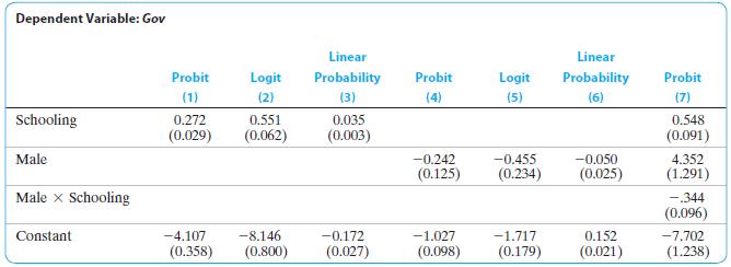
11.5 Using the results in column (7):a. Akira is a man with 10 years of schooling. What is the probability that the government will employ him?b. Jane is a woman with 12 years of schooling. What is the probability that the government will employ her?c. Does the effect of the years of schooling on
11.4 Using the results in columns (4) through (6):a. Compute the estimated probability of passing the test for men and for women.b. Are the models in (4) through (6) different? Why or why not? Dependent Variable: Gov Linear Linear Probit Logit Probability Probit Logit Probability Probit (1) (2)
11.3a. Answer (a) through (c) from Exercise 11.1 using the results in column (3).b. Sketch the predicted probabilities from the probit and linear probability in columns (1) and (3) as a function of Schoolingi for values of Schooling between 0 and 18. Do you think that the linear probability is
11.2a. Answer (a) through (c) from Exercise 11.1 using the results in column (2).b. Sketch the predicted probabilities from the probit and logit in columns(1) and (2) for values of Schooling between 0 and 18. Are the probit and logit models similar? Dependent Variable: Gov Linear Linear Probit
11.1 Using the results in column (1):a. Does the probability of working in the government depend on Schooling? Explain.b. Matthew has 16 years of schooling. What is the probability that he will pass the test?c. Christopher never went to college (12 years of schooling). What is the probability that
11.4 What measures of fit are typically used to assess binary dependent variable regression models?
11.3 What is a maximum likelihood estimation? What are the advantages of using maximum likelihood estimators such as the probit and the logit, instead of the linear probability model? How would you choose between the probit and the logit?
11.2 In Table 11.2 the estimated coefficient on black is 0.084 in column (1), 0.688 in column (2), and 0.389 in column (3). In spite of these large differences, all three models yield similar estimates of the marginal effect of race on the probability of mortgage denial. How can this be?
11.1 Suppose that a linear probability model yields a predicted value of Y that is equal to 1.3. Explain why this is nonsensical.
E10.2 Do citizens demand more democracy and political freedom as their incomes grow? That is, is democracy a normal good? On the textbook website, www.pearsonglobaleditions.com/Stock_Watson, you will find the data file Income_Democracy, which contains a panel data set from 195 countries for the
E10.1 Some U.S. states have enacted laws that allow citizens to carry concealed weapons. These laws are known as “shall-issue” laws because they instruct local authorities to issue a concealed weapons permit to all applicants who are citizens, are mentally competent, and have not been convicted
10.11 Let b nDM 1 denote the entity-demeaned estimator given in Equation (10.22), and let b nBA 1 denote the “before and after” estimator without an intercept, so that b nBA 1 = 3ni= 1(Xi2 - Xi1)(Yi2 - Yi1)4 > 3ni= 1(Xi2 - Xi1)24. Show that, if T = 2, b nDM 1 = b nBA 1 . [Hint: Use the
10.10 A researcher wants to estimate the determinants of annual earnings: age, gender, schooling, union status, occupation, and sector of employment.The researcher has been told that if they collect panel data on a large number of randomly chosen individuals over time, they will be able to regress
10.9a. In the fixed effects regression model, are the fixed entity effects, ai, consistently estimated as n¡ with T fixed? (Hint: Analyze the model with no X’s: Yit = ai + uit.)b. If n is large (say, n = 2000) but T is small (say, T = 4), do you think that the estimated values of ai are
10.8 Consider observations (Yit, Xit) from the linear panel data model Yit = Xitb1 + ai + lit + uit, where t = 1,c, T; i = 1,c, n; and ai + lit is an unobserved entityspecific time trend. How would you estimate b1?
10.7 Suppose a researcher believes that the occurrence of natural disasters, such as earthquakes, leads to increased activity in the construction industry.The researcher decides to collect province-level data on employment in the construction industry of an earthquake-prone country, and regress
10.6 Do the fixed effects regression assumptions in Key Concept 10.3 imply that cov(v it,v is) = 0 for t s in Equation (10.28)? Explain.
10.5 Consider the model with a single regressor Yit = b1X1,it + ai + lt + uit.This model also can be written as Yit = b0 + b1X1,it + d2B2t + g+ dTBTt + g2D2i + g+ gnDni + uit, where B2t = 1 if t = 2 and 0 otherwise, D2i = 1 if i = 2 and 0 otherwise, and so forth. How are the coefficients (b0, d2,c,
10.4 Using the regression in Equation (10.11), what is the slope and intercept fora. Entity 1 in time period 1?b. Entity 1 in time period 3?c. Entity 3 in time period 1?d. Entity 3 in time period 3?
10.3 Section 9.2 gave a list of five potential threats to the internal validity of a regression study. Apply that list to the empirical analysis in Section 10.6 and thereby draw conclusions about its internal validity.
10.2 Consider the binary variable version of the fixed effects model in Equation(10.11), except with an additional regressor, D1i; that is, let Yit = b0 + b1Xit + g1D1i + g2D2i + g+ gnDni + uit.a. Suppose that n = 3. Show that the binary regressors and the “constant”regressor are perfectly
10.1 This exercise refers to the drunk driving panel data regression, summarized in Table 10.1.a. New Jersey has a population of 8.85 million people. Suppose that New Jersey increased the tax on a case of beer by $2 (in 1988 dollars). Use the results in column (5) to predict the number of lives
10.4 In the context of the regression you suggested for Question 10.2, explain why the regression error for a given individual might be serially correlated.
10.3 Can the regression that you suggested in response to Question 10.2 be used to estimate the effect of gender on an individual’s earnings? Can that regression be used to estimate the effect of the national unemployment rate on an individual’s earnings? Explain.
10.2 A researcher is using a panel data set on n = 1000 workers over T = 10 years (from 2001 through 2010) that contains the workers’ earnings, gender, education, and age. The researcher is interested in the effect of education on earnings. Give some examples of unobserved person-specific
10.1 Define panel data. What is the advantage of using such data to make statistical and economic inferences? Why is it necessary to use two subscripts, i and t, to describe panel data? What does i refer to? What does t refer to?
E9.2 Use the data set Birthweight_Smoking introduced in Empirical Exercise 5.1 to answer the following questions.a. In Empirical Exercise 7.1(f), you estimated several regressions and were asked: “What is a reasonable 95% confidence interval for the effect of smoking on birth weight?”i. In
E9.1 Use the data set CPS12, described in Empirical Exercise 8.2, to answer the following questions.a. Discuss the internal validity of the regressions that you used to answer Empirical Exercise 8.2(l). Include a discussion of possible omitted variable bias, misspecification of the functional form
9.13 Assume that the regression model Yi = b0 + b1Xi + ui satisfies the least squares assumptions in Key Concept 4.3 in Section 4.4. You and a friend collect a random sample of 300 observations on Y and X.a. Your friend reports the he inadvertently scrambled the X observations for 20% of the
9.12 Consider the one-variable regression model Yi = b0 + b1Xi + ui and suppose that it satisfies the least squares assumptions in Key Concept 4.3. The regressor Xi is missing, but data on a related variable, Zi, are available, and the value of Xi is estimated usingXi = E(Xi 0Zi). Let wi = Xi -
9.11 Read the box “The Demand for Economics Journals” in Section 8.3. Discuss the internal and external validity of the estimated effect of price per citation on subscriptions.
9.10 Read the box “The Return to Education and the Gender Gap” in Section 8.3. Discuss the internal and external validity of the estimated effect of education on earnings.
9.9 Consider the linear regression of TestScore on Income shown in Figure 8.2 and the nonlinear regression in Equation (8.18). Would either of these regressions provide a reliable estimate of the effect of income on test scores? Would either of these regressions provide a reliable method for
9.8 Would the regression in Equation (9.5) be useful for predicting test scores in a school district in Massachusetts? Why or why not?
9.7 Are the following statements true or false? Explain your answer.a. “An ordinary least squares regression of Y onto X will not be internally valid if Y is correlated with the error term.”b. “If the error term exhibits heteroskedasticity, then the estimates of X will always be biased.”
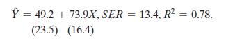
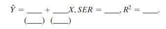
9.6 Suppose that n = 50, i.i.d. observations for (Yi, Xi) yield the following regression results:Another researcher is interested in the same regression, but makes an error when entering the data into a regression program: The researcher enters each observation twice, ending up with 100
9.5 The demand for a commodity is given by Q = b0 + b1P + u, where Q denotes quantity, P denotes price, and u denotes factors other than price that determine demand. Supply for the commodity is given by Q = g0 + g1P + v, where v denotes factors other than price that determine supply. Suppose that u
9.4 Using the regressions shown in columns (2) of Table 8.3 and 9.3, and column(2) of Table 9.2, construct a table like Table 9.3 to compare the estimated effects of a 10 percentage point increase in the students eligible for free lunch on test scores in California and Massachusetts.
9.3 Labor economists studying the determinants of women’s earnings discovered a puzzling empirical result. Using randomly selected employed women, they regressed earnings on the women’s number of children and a set of control variables (age, education, occupation, and so forth). They found that
9.2 Consider the one-variable regression model Yi = b0 + b1Xi + ui and suppose that it satisfies the least squares assumptions in Key Concept 4.3. Suppose that Yi is measured with error, so the data are Y i = Yi + wi, where wi is the measurement error, which is i.i.d. and independent of Yi and Xi.
9.1 Suppose you just read a careful statistical study of the effect of improved health of children on their test scores at school. Using data from a project in a West African district, in 2000, the study concluded that students who received multivitamin supplements performed substantially better at
9.6 A researcher estimates a regression using two different software packages.The first uses the homoskedasticity-only formula for standard errors. The second uses the heteroskedasticity-robust formula. The standard errors are very different. Which should the researcher use? Why?
9.5 Define simultaneous causality bias. Explain the potential for simultaneous causality in a study of the effects of high levels of bureaucratic corruption on national income.
9.4 What is sample selection bias? Suppose you read a study using data on college graduates of the effects of an additional year of schooling on earnings.What is the potential sample selection bias?
9.3 What is the effect of measurement error in Y? How is this different from the effect of measurement error in X?
9.2 Key Concept 9.2 describes the problem of variable selection in terms of a trade-off between bias and variance. What is this trade-off? Why could including an additional regressor decrease bias? Increase variance?
9.1 Is it possible for an econometric study to have internal validity but not external validity?
E8.2 On the text website www.pearsonglobaleditions.com/Stock_Watson you will find a data file CPS12, which contains data for full-time, full-year workers, ages 25–34, with a high school diploma or B.A./B.S. as their highest degree. A detailed description is given in CPS12_Description, also
E8.1 Lead is toxic, particularly for young children, and for this reason government regulations severely restrict the amount of lead in our environment.But this was not always the case. In the early part of the 20th century, the underground water pipes in many U.S. cities contained lead, and lead
8.12 The discussion following Equation (8.28) interprets the coefficient on interacted binary variables using the conditional mean zero assumption.This exercise shows that interpretation also applies under conditional mean independence. Consider the hypothetical experiment in Exercise 7.11.a.
8.11 Derive the expressions for the elasticities given in Appendix 8.2 for the linear and log-log models. (Hint: For the log-log model, assume that u and X are independent, as is done in Appendix 8.2 for the log-linear model.)
8.10 Consider the regression model Yi = b0 + b1X1i + b2X2i + b3(X1i * X2i) +ui. Use Key Concept 8.1 to show:a. Y>X1 = b1 + b3X2 (effect of change in X1, holding X2 constant).b. Y>X2 = b2 + b3X1 (effect of change in X2, holding X1 constant).c. If X1 changes by X1 and X2 changes by X2, then Y
8.9 Explain how you would use Approach #2 from Section 7.3 to calculate the confidence interval discussed below Equation (8.8). [Hint: This requires estimating a new regression using a different definition of the regressors and the dependent variable. See Exercise (7.9).]
8.8 X is a continuous variable that takes on values between 5 and 100. Z is a binary variable. Sketch the following regression functions (with values of X between 5 and 100 on the horizontal axis and values of Y n on the vertical axis):a. Y n= 2.0 + 3.0 * ln(X).b. Y n= 2.0 - 3.0 * ln(X).c. i. Y n=
8.7 This problem is inspired by a study of the “gender gap” in earnings in top corporate jobs [Bertrand and Hallock (2001)]. The study compares total compensation among top executives in a large set of U.S. public corporations in the 1990s. (Each year these publicly traded corporations must
8.6 Refer to Table 8.3.a. A researcher suspects that the effect of %Eligible for subsidized lunch has a nonlinear effect on test scores. In particular, he conjectures that increases in this variable from 10% to 20% have little effect on test scores but that changes from 50% to 60% have a much
8.5 Read the box “The Demand for Economics Journals” in Section 8.3.a. The box reaches three conclusions. Looking at the results in the table, what is the basis for each of these conclusions?b. Using the results in regression (4), the box reports that the elasticity of demand for an 80-year-old
8.4 Read the box “The Return to Education and the Gender Gap” in Section 8.3.a. Consider a man with 16 years of education and 2 years of experience who is from a western state. Use the results from column (4)of Table 8.1 and the method in Key Concept 8.1 to estimate the expected change in the
8.3 After reading this chapter’s analysis of test scores and class size, an educator comments, “In my experience, student performance depends on class size, but not in the way your regressions say. Rather, students do well when class size is less than 20 students and do very poorly when class
8.2 Suppose a researcher collects data on houses that have been sold in a particular neighborhood over the past year, and obtains the regression results in the table shown below.a. Using the results in column (1), what is the expected change in price of building a 1500-square-foot addition to a
8.1 Sales of a company is $243 million in 2013, and it increases to $250 million in 2014.a. Compute the percentage increase in sales, using the usual formula 100 * (Sales2014 - Sales2013)Sales2013 . Compare this value to the approximation.100 * 3ln(Sales2014) - ln(Sales2013)4.b. Repeat (a),
8.6 What types of independent variables—binary or continuous—may interact with one another in a regression? How do you interpret the coefficient on the interaction between two continuous regressors and two binary regressors?
8.5 Suppose that in Exercise 8.2 you thought that the value of b2 was not constant but rather increased when K increased. How could you use an interaction term to capture this effect?
8.4 Suppose the regression in Equation (8.30) is estimated using LoSTR and LoEL in place of HiSTR and HiEL, where LoSTR = 1 - HiSTR is an indicator for a low-class-size district and LoEL = 1 - HiEL is an indicator for a district with a low percentage of English learners. What are the values of the
8.3 How is the slope coefficient interpreted in a log-linear model, where the dependent variable is (i) in logarithms but the independent variable is not, (ii)in a linear-log model, (iii) in a log-log model?
8.2 A “Cobb–Douglas” production function relates production (Q) to factors of production, capital (K), labor (L), and raw materials (M), and an error term u using the equation Q = lKb1Lb2Mb3eu, where l, b1, b2, and b3 are production parameters. Suppose that you have data on production and the
8.1 A researcher tells you that there are non-linearities in the relationship between wages and years of schooling. What does this mean? How would you test for non-linearities in the relationship between wages and schooling? How would you estimate the rate of change in wages with respect to years
E7.2 In the empirical exercises on earning and height in Chapters 4 and 5, you estimated a relatively large and statistically significant effect of a worker’s height on his or her earnings. One explanation for this result is omitted variable bias:Height is correlated with an omitted factor that
E7.1 Use the Birthweight_Smoking data set introduced in Empirical Exercise E5.3 to answer the following questions. To begin, run three regressions:(1) Birthweight on Smoker(2) Birthweight on Smoker, Alcohol, and Nprevist(3) Birthweight on Smoker, Alcohol, Nprevist, and Unmarrieda. What is the value
7.11 A school district undertakes an experiment to estimate the effect of class size on test scores in second-grade classes. The district assigns 50% of its previous year’s first graders to small second-grade classes (18 students per classroom) and 50% to regular-size classes (21 students per
7.10 Equations (7.13) and (7.14) show two formulas for the homoskedasticityonly F-statistic. Show that the two formulas are equivalent.
7.9 Consider the regression model Yi = b0 + b1X1i + b2X2i + ui. Use Approach#2 from Section 7.3 to transform the regression so that you can use a t-statistic to testa. b1 = b2.b. b1 + 2b2 = 0.c. b1 + b2 = 1. (Hint: You must redefine the dependent variable in the regression.)
7.8 Referring to the table on page 292 used for exercises 7.1–7.6:a. Construct the R2 for each of the regressions.b. Show how to construct the homoskedasticity-only F-statistic for testing b4 = b5 = b6 = 0 in the regression shown in column (3).c. Test b4 = b5 = b6 = 0 in the regression shown in
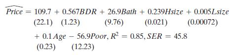
7.7 Question 6.5 reported the following regression (where standard errors have been added):a. Is the coefficient on BDR statistically significantly different from zero?b. Typically four-bedroom houses sell for more than three-bedroom houses. Is this consistent with your answer to (a), and with the
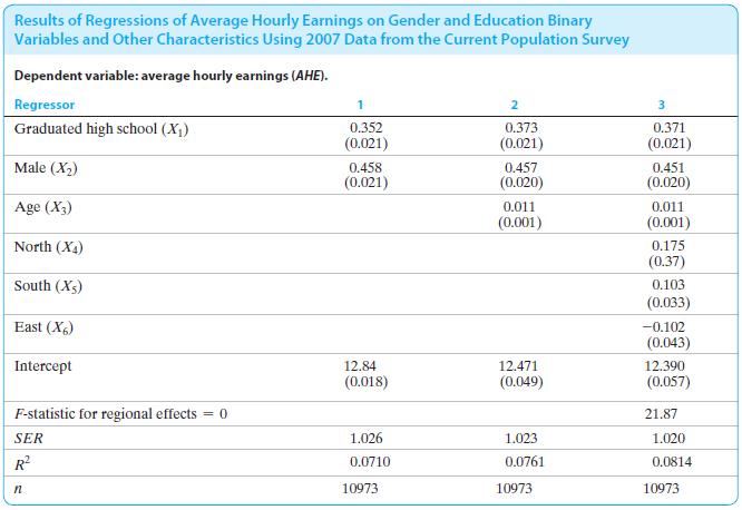
7.6 In all the regressions, the coefficient of High school is positive, large, and statistically significant. Do you believe this provides strong statistical evidence of the high returns to schooling in the labor market?The data set consists of information on over 10000 full-time, full-year
7.5 The regression shown in column (2) was estimated again, this time using data from 1993 (5000 observations selected at random and converted into 2007 units using the consumer price index). The results areComparing this regression to the regression for 2012 shown in column (2), was there a
7.4 Using the regression results in column (3):a. Are there important regional differences? Use an appropriate hypothesis test to explain your answer.b. Juan is a 32-year-old male high school graduate from the North. Ali is a 32-year-old male college graduate from the West. Mayank is a 32-year-old
7.3 Using the regression results in column (2):a. Is age an important determinant of earnings? Use an appropriate statistical test and/or confidence interval to explain your answer.b. Alvo is a 30-year-old male college graduate. Kal is a 40-year-old male college graduate. Construct a 95% confidence
7.2 Using the regression results in column (1):a. Is the college–high school earnings difference, estimated from this regression, statistically significant at the 5% level? Construct a 95%confidence interval of the difference.b. Is the male–female earnings difference, estimated from this
7.1 Add * (5%) and ** (1%) to the table to indicate the statistical significance of the coefficients.The data set consists of information on over 10000 full-time, full-year workers. The highest educational achievement for each worker was either a high school diploma or a bachelor’s degree. The
7.3 What is a control variable, and how does it differ from a variable of interest?Looking at Table 7.1, which variables are control variables? What is the variable of interest? Do coefficients on control variables measure causal effects? Explain.
7.2 Describe the recommended approach towards determining model specification.How does the R2 help in determining an appropriate model? Is the ideal model the one with the highest R2? Should a regressor be included in the model if it increases the model R2?
7.1 What is a joint hypothesis? Explain how an F-statistic is constructed to test a joint hypothesis. What is the hypothesis that is tested by constructing the overall regression F-statistic in the multiple regression model Yi = b0 + b1X1i + b2X2i + ui? Explain, using the concepts of restricted and
E6.2 Using the data set Growth described in Empirical Exercise E4.1, but excluding the data for Malta, carry out the following exercises.a. Construct a table that shows the sample mean, standard deviation, and minimum and maximum values for the series Growth, Trade-Share, YearsSchool, Oil,
E6.1 Use the Birthweight_Smoking data set introduced in Empirical Exercise E5.3 to answer the following questions.a. Regress Birthweight on Smoker. What is the estimated effect of smoking on birth weight?b. Regress Birthweight on Smoker, Alcohol, and Nprevist.i. Using the two conditions in Key
6.11 (Requires calculus) Consider the regression model Yi = b1X1i + b2X2i + ui for i = 1,c, n. (Notice that there is no constant term in the regression.)Following analysis like that used in Appendix (4.2):a. Specify the least squares function that is minimized by OLS.b. Compute the partial
6.10 (Yi, X1i, X2i) satisfy the assumptions in Key Concept 6.4; in addition, var(ui X1i, X2i) = 4 and var(X1i) = 6. A random sample of size n = 400 is drawn from the population.a. Assume that X1 and X2 are uncorrelated. Compute the variance of b n1.[Hint: Look at Equation (6.17) in Appendix
6.9 (Yi, X1i, X2i) satisfy the assumptions in Key Concept 6.4. You are interested in b1, the causal effect of X1 on Y. Suppose that X1 and X2 are uncorrelated.You estimate b1 by regressing Y onto X1 (so that X2 is not included in the regression). Does this estimator suffer from omitted variable
6.8 A government study found that people who eat chocolate frequently weigh less than people who don’t. Researchers questioned 1000 individuals from California between the ages of 20 and 85 about their eating habits, and measured their weight and height. On average, participants ate chocolate

Showing 3200 - 3300 of 4105

First
26
27
28
29
30
31
32
33
34
35
36
37
38
39
40
Last

Step by Step Answers

Services

Sitemap
Fun
Definitions
Become Tutor
Used Textbooks
Study Help Categories
Recent Questions
Expert Questions
Campus Wear
Sell Your Books

Company Info

Security
Copyrights
Privacy Policy
Terms & Conditions
SolutionInn Fee
Scholarship
Online Quiz
Give Feedback, Get Rewards

Get In Touch

About Us
Contact Us
Career
Jobs
FAQ
Student Discount
Campus Ambassador

Secure Payment

Download Our App

© 2026 SolutionInn. All Rights Reserved