New Semester
Started
Get
50% OFF
Study Help!
--h --m --s
Claim Now
Question Answers
Textbooks
Find textbooks, questions and answers
Oops, something went wrong!
Change your search query and then try again
S
Books
FREE
Study Help
Expert Questions
Accounting
General Management
Mathematics
Finance
Organizational Behaviour
Law
Physics
Operating System
Management Leadership
Sociology
Programming
Marketing
Database
Computer Network
Economics
Textbooks Solutions
Accounting
Managerial Accounting
Management Leadership
Cost Accounting
Statistics
Business Law
Corporate Finance
Finance
Economics
Auditing
Tutors
Online Tutors
Find a Tutor
Hire a Tutor
Become a Tutor
AI Tutor
AI Study Planner
NEW
Sell Books
Search
Search
Sign In
Register
study help
business
econometrics
Basic Econometrics 5th edition Damodar N. Gujrati, Dawn C. Porter - Solutions
Omission of a variable in the K-variable regression model. Refer to Eq. (13.3.3), which shows the bias in omitting the variable X3 from the model Yi = β1+β2X2i + β3X3i + ui . This can be generalized as follows: In the k-variable model Yi = β1 + β2X2i + · · ·+βk Xki + ui , suppose we omit
What is meant by intrinsically linear and intrinsically nonlinear regression models?
Since the error term in the Cobb–Douglas production function can be entered multiplicatively or additively, how would you decide between the two?
What is the difference between OLS and nonlinear least-squares (NLLS) estimation?
The relationship between pressure and temperature in saturated steam can be expressed as:*where Y = pressure and t = temperature. Using the method of nonlinear least squares (NLLS), obtain the normal equations for this model. Y = B1(10)P2t/(y+1) + U:
State whether the following statements are true or false.a. Statistical inference in NLLS regression cannot be made on the basis of the usual t, F, and χ2 tests even if the error term is assumed to be normally distributed.b. The coefficient of determination (R2) is not a particularly meaningful
How would you linearize the CES production function discussed in the chapter? Show the necessary steps.
Models that describe the behavior of a variable over time are called growth models. Such models are used in a variety of fields, such as economics, biology, botany, ecology, and demography. Growth models can take a variety of forms, both linear and nonlinear. Consider the following models, where Y
The true model isY*i = β1 + βX*i + ui €¦€¦€¦€¦€¦€¦€¦€¦€¦€¦€¦.. (1)But because of errors of measurement you estimateYi = α1 +
Critically evaluate the following view expressed by Leamer:My interest in metastatistics [i.e., theory of inference actually drawn from data] stems from my observations of economists at work. The opinion that econometric theory is irrelevant is held by an embarrassingly large share of the economic
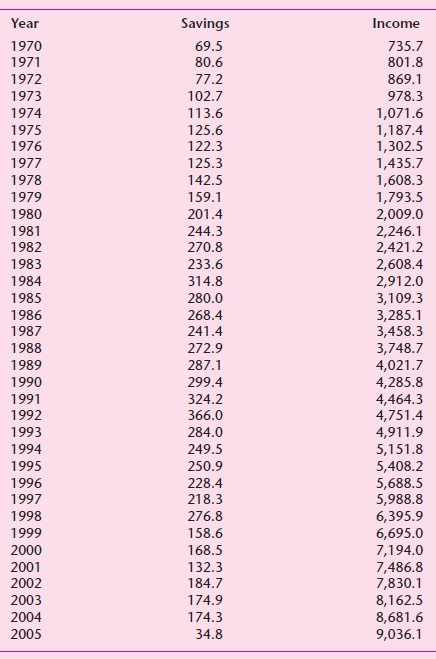
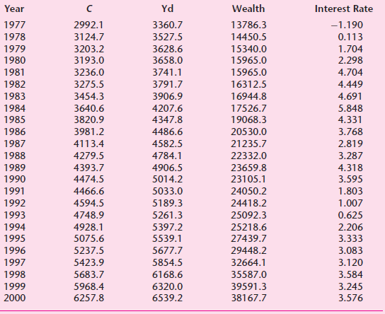
Refer to Table 8.11, which gives data on personal savings (Y) and personal disposable income (X) for the period 1970–2005. Now consider the following models: Model A: Yt = α1 + α2Xt + α3Xt−1 + utModel B: Yt = β1 + β2Xt + β3Yt−1 + uta. How would you choose
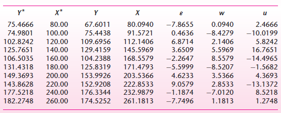
Monte Carlo experiment.* Ten individuals had weekly permanent income as follows: $200, 220, 240, 260, 280, 300, 320, 340, 380, and 400. Permanent consumption (Y∗i) was related to permanent income X∗i asY∗I = 0.8X∗i
Continue with Exercise 13.21. Strictly for pedagogical purposes, assume that model (2) is the true demand function.a. If we now estimate model (1), what type of specification error is committed in this instance?b. What are the theoretical consequences of this specification error? Illustrate with
Use the data for the demand for chicken given in Exercise 7.19. Suppose you are told that the true demand function isln Yt = β1 + β2 ln X2t + β3 ln X3t + β6 ln X6t + ut
State with reason whether the following statements are true or false.†a. An observation can be influential but not an outlier.b. An observation can be an outlier but not influential.c. An observation can be both influential and an outlier.d. If in the model Yi = β1 + β2Xi + β3X2i+ uiβ3 turns
Refer to the St. Louis model discussed in the text. Keeping in mind the problems associated with the nested F test, critically evaluate the results presented in regression (13.8.4).
According to Blaug, “There is no logic of proof but there is logic of disproof.” What does he mean by this?
Evaluate the following statement made by Henry Theil:*Given the present state of the art, the most sensible procedure is to interpret confidence coefficients and significance limits liberally when confidence intervals and test statistics are computed from the final regression of a regression
Refer to the demand function for chicken estimated in Eq. (8.6.23). Considering the attributes of a good model discussed in Section 13.1, could you say that this demand function is “correctly” specified?
Suppose that the true model isYi = β1 Xi + ui ……………… (1)but instead of fitting this regression through the origin you routinely fit the usual intercept present model:Yi = α0 + α1Xi + vi ………………. (2)Assess the consequences of this specification error.
Continue with Exercise 13.2 but assume that it is model (2) that is the truth. Discuss the consequences of fitting the mis-specified model (1).In exercise 13.2Suppose that the true model isYi = β1 Xi + ui ……………… (1)but instead of fitting this regression through the origin you routinely
Suppose that the “true” model isYi = β1 + β2X2i + uibut we add an “irrelevant” variable X3 to the model (irrelevant in the sense that the true β3 coefficient attached to the variable X3 is zero) and estimateYi = β1 + βX2i + β3X3i + via. Would the R2 and the adjusted R2 for model (2)
Consider the following “true” (Cobb–Douglas) production function:ln Yi = α0 + α1 ln L1i + α2 ln L2i + α3 ln Ki + uiwhereY = outputL1 = production laborL2 = nonproduction laborK = capitalBut suppose the regression actually used in empirical investigation isln Yi = β0 + β1 ln L1i + β2 ln
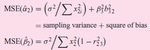
Refer to Eqs. (13.3.4) and (13.3.5). As you can see, α̂2, although biased, has a smaller variance than β̂2, which is unbiased. How would you decide on the trade-off between bias and smaller variance? MSE(â2) = = (0/E3) + B}b3: = sampling variance
Show that β estimated from either Eq. (13.5.1) or Eq. (13.5.3) provides an unbiased estimate of true β.
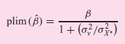
Following Friedman€™s permanent income hypothesis, we may writeYˆ—i = α + βXˆ—iwhere Yˆ—i = €œpermanent€ consumption expenditure and Xˆ—i = €œpermanent€ income. Instead of observing
Consider the modelYi = β1 + β2X2i + ui…………….. (1)To find out whether this model is mis-specified because it omits the variable X3 from the model, you decide to regress the residuals obtained from model (1) on the variable X3 only. (There is an intercept in this regression.) The Lagrange
Consider the modelYi = β1 + β2X∗i + uiIn practice we measure X∗i by Xi such thata. Xi = X∗i + 5b. Xi = 3X∗ic. Xi = (X∗i + εi ), where εi is a purely random term with the usual properties.What will be the effect of these measurement errors on estimates of true β1 and β2?
Refer to the regression Eqs. (13.3.1) and (13.3.2). In a manner similar to Eq. (13.3.3) show thatE(α̂1) = β1 + β3(X̅3 − b32X̅2)where b32 is the slope coefficient in the regression of the omitted variable X3 on the included variable X2.
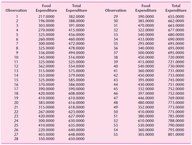
Food expenditure in India. In the following table we have given data on expenditure on food and total expenditure for 55 families in India.a. Regress expenditure on food on total expenditure, and examine the residuals obtained from this regression.b. Plot the residuals obtained in (a) against total
Estimating ρ: The Cochrane–Orcutt (C–O) iterative procedure. As an illustration of this procedure, consider the two-variable model:Yt = β1 + β2Xt + ut …………………….. (1)and the AR(1) schemeut = ρut−1 + εt , −1 < ρ < 1 ……………. (2)Cochrane and Orcutt then
Return to the R&D example discussed in Section 11.7 (Exercise 11.10). Repeat the example using profits as the regressor. A priori, would you expect your results to be different from those using sales as the regressor? Why or why not?
Although log models as shown in Eq. (11.6.12) often reduce heteroscedasticity, one has to pay careful attention to the properties of the disturbance term of such models. For example, the modelYi = β1Xβ2i ui ……………………………………………. (1)can be written asln Yi = ln β1 +
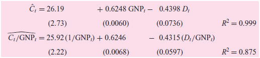
For pedagogic purposes Hanushek and Jackson estimate the following model:Ct = β1 + β2GNPt + β3Dt + ui €¦€¦€¦€¦€¦€¦€¦€¦€¦.. (1)where Ct = aggregate private
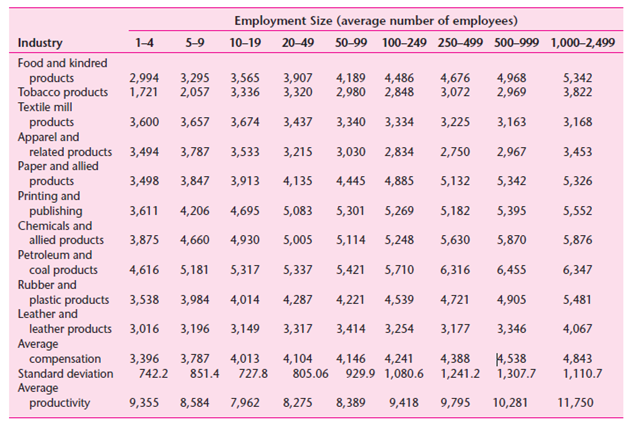
For the data given in the following table, regress average compensation Y on average productivity X, treating employment size as the unit of observation. Interpret your results, and see if your results agree with those given in Eq. (11.5.3).a. From the preceding regression obtain the residuals
The following table gives data on the sales/cash ratio in U.S. manufacturing industries classified by the asset size of the establishment for the period 1971–I to 1973–IV. (The data are on a quarterly basis.) The sales/cash ratio may be regarded as a measure of income velocity in the corporate
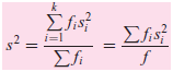
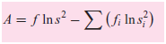
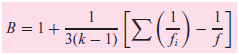
Bartlett€™s homogeneity-of-variance test.* Suppose there are k independent sample variances s21, s22, . . . , s2kwith f1, f2, . . . , fkdf, each from populations which are normally distributed with mean μ and variance σ2i. Suppose further that we want to test the
Consider the following regression-through-the origin model:Yi = βXi + ui, for i = 1, 2You are told that u1 ∼ N(0, σ2) and u2 ∼ N(0, 2σ2) and that they are statistically independent. If X1=+1 and X2=−1, obtain the weighted least-squares (WLS) estimate of β and its variance.
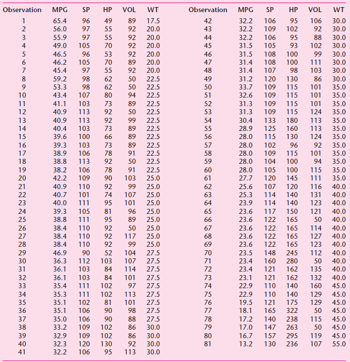
The following table gives data on 81 cars about MPG (average miles per gallons), HP (engine horsepower), VOL (cubic feet of cab space), SP (top speed, miles per hour), and WT (vehicle weight in 100 lbs.).a. Consider the following model:MPGi = β1 + β2SPi + β3HPi + β4WTi + uiEstimate the
Repeat Exercise 11.16, but this time regress the logarithm of expenditure on food on the logarithm of total expenditure. If you observe heteroscedasticity in the linear model of Exercise 11.16 but not in the log€“linear model, what conclusion do you draw? Show all the necessary
A shortcut to White’s test. As noted in the text, the White test can consume degrees of freedom if there are several regressors and if we introduce all the regressors, their squared terms, and their cross products. Therefore, instead of estimating regressions like Eq. (11.5.22), why not simply
State whether the following statements are true or false. Briefly justify your answer.a. When autocorrelation is present, OLS estimators are biased as well as inefficient.b. The Durbin–Watson d test assumes that the variance of the error term ut is homoscedastic.c. The first-difference
Given a sample of 50 observations and 4 explanatory variables, what can you say about autocorrelation if (a) d = 1.05? (b) d = 1.40? (c) d = 2.50? (d) d = 3.97?
In studying the movement in the production workers’ share in the value added (i.e., labor’s share), the following models were considered by Gujarati:*Model A: Yt = β0 + β1t + utModel B: Yt = α0 + α1t + α2t2 + utwhere Y = labor’s share and t = time. Based on annual data for 1949–1964,
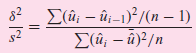
Detecting autocorrelation: von Neumann ratio test.* Assuming that the residual ûtare random drawings from normal distribution, von Neumann has shown that for large n, the ratiocalled the von Neumann ratio, is approximately normally distributed with meanand variancea. If n is
In a sequence of 17 residuals, 11 positive and 6 negative, the number of runs was 3. Is there evidence of autocorrelation? Would the answer change if there were 14 runs?
Theil€“Nagar Ï estimate based on d statistic. Theil and Nagar have suggested that, in small samples, instead of estimating Ï as (1 ˆ’ d/2), it should be estimated aswhere n = total number of observations, d = Durbin€“Watson d, and k = number of
Refer to Exercise 7.19 about the demand function for chicken in the United States.a. Using the log–linear, or double-log, model, estimate the various auxiliary regressions. How many are there?b. From these auxiliary regressions, how do you decide which regressor(s) is highly collinear? Which test
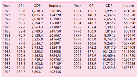
The following table gives data on imports, GDP, and the Consumer Price Index (CPI) for the United States over the period 1975€“2005. You are asked to consider the following model:ln Importst = β1 + β2 lnGDPt + β3 ln CPIt + uta. Estimate the parameters
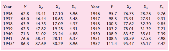
Klein and Goldberger attempted to fit the following regression model to the U.S. economy:Yi = β1 + β2X2i + β3X3i + β4X4i + uiwhere Y = consumption, X2 = wage income, X3 = nonwage, nonfarm income, and X4 = farm income. But since X2, X3, and X4 are
Critically evaluate the following statements:a. “In fact, multicollinearity is not a modeling error. It is a condition of deficient data.”b. “If it is not feasible to obtain more data, then one must accept the fact that the data one has contain a limited amount of information and must
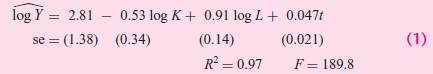
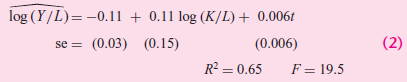
From the annual data for the U.S. manufacturing sector for 1899€“1922, Dougherty obtained the following regression results:where Y = index of real output, K = index of real capital input, L = index of real labor input, t = time or trend.Using the same data, he also obtained the following
For the k-variable regression model, it can be shown that the variance of the kth (k = 2, 3, . . . , K) partial regression coefficient given in Eq. (7.5.6) can also be expressed aswhere σ2y = variance of Y, σ2k = variance of the kth explanatory variable, R2k =
Verify that the standard errors of the sums of the slope coefficients estimated from Eqs. (10.5.6) and (10.5.7) are, respectively, 0.1549 and 0.1825.
Using Eqs. (7.4.12) and (7.4.15), show that when there is perfect collinearity, the variances of β̂2 and β̂3 are infinite.
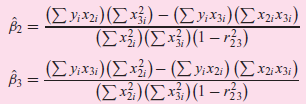
Show that Eqs. (7.4.7) and (7.4.8) can also be expressed aswhere r23 is the coefficient of correlation between X2 and X3. (ΣΥ) (Σx)-(Σy) (Σ3) β- ΙΣ3/Σ-r3) (ΣΥκε) (Σx) -(Συ) (Σ) β [Σ3) (Σ) 1-5)
Consider the following model:GNPt = β1 + β2Mt + β3Mt−1 + β4(Mt −Mt−1) + utwhere GNPt = GNP at time t,Mt = money supply at time t, Mt−1 = money supply at time (t − 1), and (Mt −Mt−1) = change in the money supply between time t and time (t − 1). This model thus postulates that the
Orthogonal explanatory variables. Suppose in the modelYi = β1 + β2X2i + β3X3i + · · ·+βk Xki + uiX2 to Xk are all uncorrelated. Such variables are called orthogonal variables. If this is the case:a. What will be the structure of the (X'X) matrix?b. How would you obtain β̂ = (X'X)−1X'y?c.
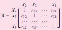
Consider the following correlation matrix:Describe how you would find out from the correlation matrix whether (a) There is perfect collinearity, (b) There is less than perfect collinearity, (c) The X€™s are uncorrelated.You may use |R| to answer these questions, where |R|
Using matrix notation, it can be shownvar–cov (β̂) = σ2(X'X)−1What happens to this var–cov matrix:a. When there is perfect multicollinearity?b. When collinearity is high but not perfect?
In matrix notation it can be shown (see Appendix C) thatβ̂ = (X'X)−1X'ya. What happens to β̂ when there is perfect collinearity among the X’s?b. How would you know if perfect collinearity exists?
Suppose all the zero-order correlation coefficients of X1(= Y), X2, . . . , Xk are equal to r.a. What is the value of R21.23 . . . k?b. What are the values of the first-order correlation coefficients?
Reestimate the model in Exercise 9.22 by adding the regressor, expenditure on durable goods.a. Is there a difference in the regression results you obtained in Exercise 9.22 and in this exercise? If so, what explains the difference?b. If there is seasonality in the durable goods expenditure data,
Consider the following model:Yi = β1 + β2Di + uiWhereDi = 0 for the first 20 observations and Di = 1 for the remaining 30 observations. You are also told that var (u2i) = 300.a. How would you interpret β1 and β2?b. What are the mean values of the two groups?c. How would you compute the variance
From data for 101 countries on per capita income in dollars (X) and life expectancy in years (Y) in the early 1970s, Sen and Srivastava obtained the following regression results: Ŷi = −2.40 + 9.39 ln Xi − 3.36 [Di (ln Xi − 7)]se = (4.73) (0.859)
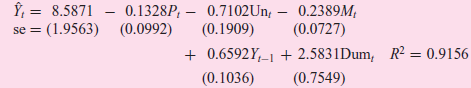
To assess the effect of the Fed€™s policy of deregulating interest rates beginning in July 1979, Sidney Langer, a student of mine, estimated the following model for the quarterly period of 1975€“III to 1983€“II.WhereY = 3-month Treasury bill rateP = expected rate of
In regression (7.9.4), we presented the results of the Cobb–Douglas production function fitted to the manufacturing sector of all 50 states and Washington, DC, for 2005. On the basis of that regression, find out if there are constant returns to scale in that sector, usinga. The t test given in
Establish statements (8.6.11) and (8.6.12).
Show that the F ratio of Eq. (8.4.16) is equal to the F ratio of Eq. (8.4.18). (ESS/TSS = R2.)
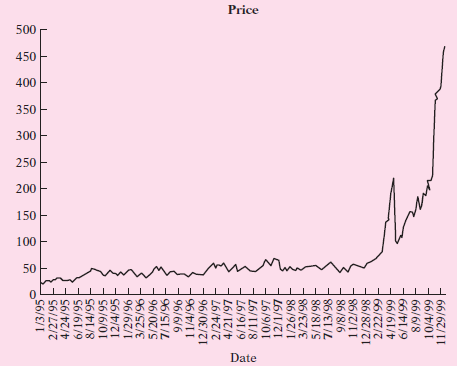
Estimating Qualcomm stock prices. As an example of the polynomial regression, consider data on the weekly stock prices of Qualcomm, Inc., a digital wireless telecommunications designer and manufacturer over the time period of 1995 to 2000. The full data can be found on the textbook€™s
Repeat Exercise 3.25, replacing math scores for reading scores.
Given the assumptions in column 1 of the table, show that the assumptions in column 2 are equivalent to them.Assumptions of the Classical Model(1)…………………………….................... (2)E(ui\Xi) ………………………..................E (Yi\Xi) = β2 + β2XCov (ui, uj) = 0 i
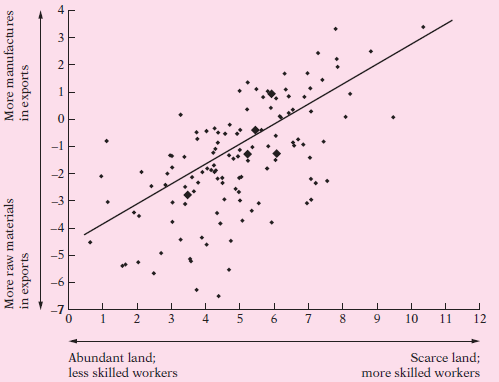
From the scattergram given in Figure 2.9, what general conclusions do you draw? What is the economic theory that underlies this scattergram? 10 11 12 6. Scarce land; Abundant land; less skilled workers more skilled workers More manufactu res More raw materials in exports in exports 2. 3. 2. 3. 4.
Estimating ρ: The Hildreth–Lu scanning or search procedure.* Since in the first order autoregressive schemeut = ρut−1 + εtρ is expected to lie between −1 and +1, Hildreth and Lu suggest a systematic “scanning’’ or search procedure to locate it. They recommend selecting ρ between
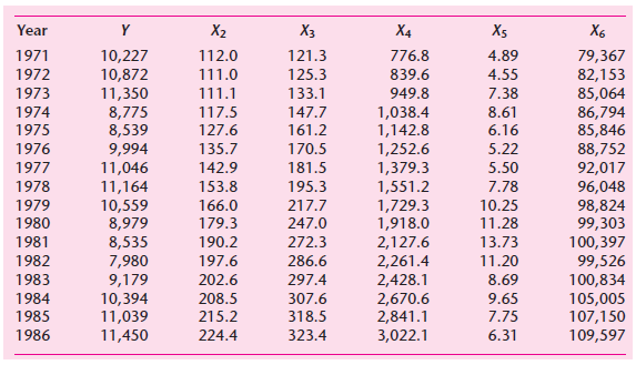
The following table gives data on new passenger cars sold in the United States as a function of several variables.a. Develop a suitable linear or log€“linear model to estimate a demand function for automobiles in the United States.b. If you decide to include all the regressors given in
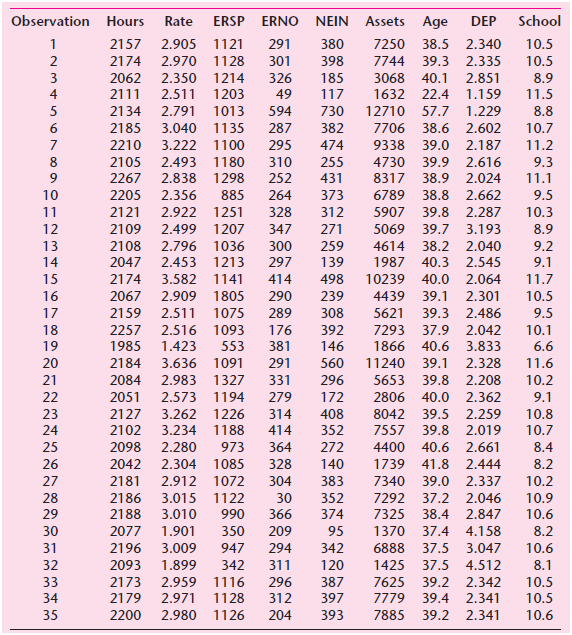
To assess the feasibility of a guaranteed annual wage (negative income tax), the Rand Corporation conducted a study to assess the response of labor supply (average hours of work) to increasing hourly wages.* The data for this study were drawn from a national sample of 6,000 households with a male
Refer to the Longley data given in Section 10.10. Repeat the regression given in the table there by omitting the data for 1962; that is, run the regression for the period 1947–1961. Compare the two regressions. What general conclusion can you draw from this exercise?
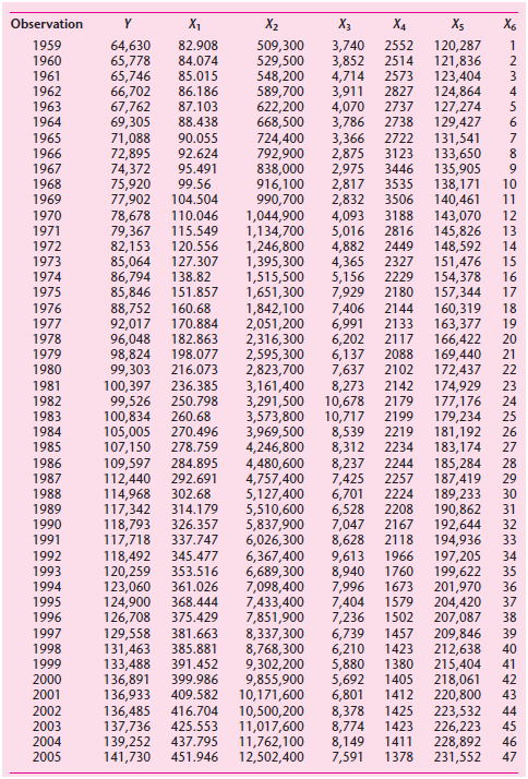
Updated Longley data. We have extended the data given in Section 10.10 to include observations from 1959€“2005. The new data are in the following table. The data pertain to Y = number of people employed, in thousands; X1= GNP implicit price deflator; X2= GNP, millions of dollars; X3=
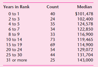
The following table gives data on median salaries of full professors in statistics in research universities in the United States for the academic year 2007.a. Plot median salaries against years in rank (as a measure of years of experience). For the plotting purposes, assume that the median salaries
You are given the following data:RSS1 based on the first 30 observations = 55, df = 25RSS2 based on the last 30 observations = 140, df = 25Carry out the Goldfeld–Quandt test of heteroscedasticity at the 5 percent level of significance.
The following table gives data on percent change per year for stock prices (Y) and consumer prices (X) for a cross section of 20 countries.a. Plot the data in a scattergram.b. Regress Y on X and examine the residuals from this regression. What do you observe?c. Since the data for Chile seem
Table 11.10 from the website gives salary and related data on 447 executives of Fortune 500 companies. Data include salary = 1999 salary and bonuses; totcomp = 1999 CEO total compensation; tenure = number of years as CEO (0 if less than 6 months); age = age of CEO; sales = total 1998 sales revenue
State with brief reason whether the following statements are true, false, or uncertain:a. In the presence of heteroscedasticity OLS estimators are biased as well as inefficient.b. If heteroscedasticity is present, the conventional t and F tests are invalid.c. In the presence of heteroscedasticity
In a regression of average wages (W, $) on the number of employees (N) for a random sample of 30 firms, the following regression results were obtained: Ŵ = 7.5 + 0.009N …………………………… (1) t = n.a. (16.10)
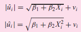
a. Can you estimate the parameters of the modelsby the method of ordinary least squares? Why or why not?b. If not, can you suggest a method, informal or formal, of estimating the parameters of such models? Jû¡| = /B1 + B2X; + v; VB1 + B2X} + v; Bi + B2X + vi J |û¡|=
Prove that if wi = w, a constant, for each i, β∗2 and β̂2 as well as their variance are identical.
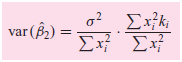
Refer to formulas (11.2.2) and (11.2.3). Assumeσ2i = σ2kiwhere σ2 is a constant and where ki are known weights, not necessarily all equal.Using this assumption, show that the variance given in Eq. (11.2.2) can be expressed asThe first term on the right side is the
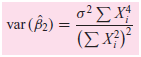
In the modelYi = β2Xi + ui (There is no intercept)you are told that var (ui) = σ2X2i . Show that 2ΣΧΧ (ΣΧ) var (B2) =
Consider the three-variable linear regression model discussed in this chapter.a. Suppose you multiply all the X2 values by 2. What will be the effect of this rescaling, if any, on the estimates of the parameters and their standard errors?b. Now instead of (a), suppose you multiply all the Y values
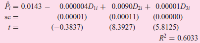
Determinants of price per ounce of cola. Cathy Schaefer, a student of mine, estimated the following regression from cross-sectional data of 77 observations:Pi = β0 + β1D1i + β2D2i + β3D3i + μiWherePi = price per ounce of colaD1i = 001 if
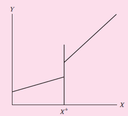
Refer to the piecewise regression discussed in the text. Suppose there not only is a change in the slope coefficient at Xˆ—but also the regression line jumps, as shown in the following Figure. How would you modify Eq. (9.8.1) to take into account the jump in the regression line at
In his study on the labor hours spent by the FDIC (Federal Deposit Insurance Corporation) on 91 bank examinations, R. J. Miller estimated the following function:WhereY = FDIC examiner labor hoursX1 = total assets of bankX2 = total number of offices in bankX3 = ratio of classified loans to total
Refer to the U.S. savings–income example discussed in Section 9.5.a. How would you obtain the standard errors of the regression coefficients given in Eqs. (9.5.5) and (9.5.6), which were obtained from the pooled regression (9.5.4)?b. To obtain numerical answers, what additional information, if
Refer to regression (9.7.3). How would you test the hypothesis that the coefficients of D2 and D3 are the same? And that the coefficients of D2 and D4 are the same? If the coefficient of D3 is statistically different from that of D2 and the coefficient of D4 is different from that of D2, does that
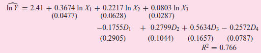
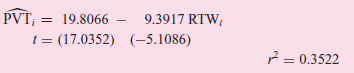
To assess the effect of state right-to-work laws (which do not require membership in the union as a precondition of employment) on union membership, the following regression results were obtained, from the data for 50 states in the United States for 1982:where PVT = percentage of private sector
In the following regression model:Yi = β1 + β2Di + uiY represents hourly wage in dollars and D is the dummy variable, taking a value of 1 for a college graduate and a value of 0 for a high-school graduate. Using the OLS formulas given in Chapter 3, show that β̂1 = Y̅hg and β̂2 = Y̅cg –
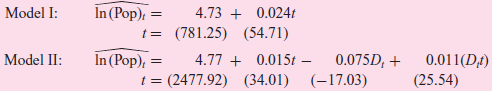
To study the rate of growth of population in Belize over the period 1970€“1992, Mukherjee et al. estimated the following models:where Pop = population in millions, t = trend variable, Dt = 1 for observations beginning in 1978 and 0 before 1978, and ln stands for natural logarithm.a. In
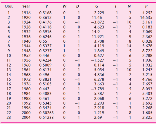
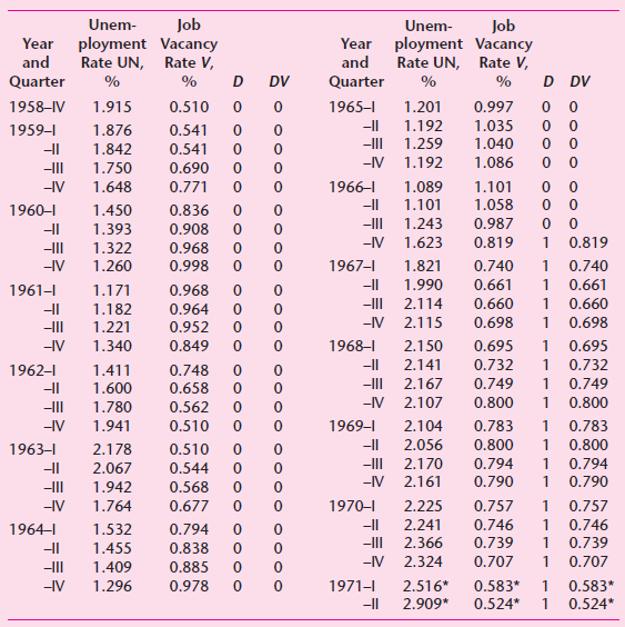
Using the data given in the following, test the hypothesis that the error variances in the two subperiods 1958€“IV to 1966€“III and 1966€“IV to 1971€“II are the same. Job ployment Vacancy Rate UN, Rate V, Unem- Job ployment Vacancy Rate UN, Rate V, Unem- Year
Using the methodology discussed in Chapter 8, compare the unrestricted and restricted regressions (9.7.3) and (9.7.4); that is, test for the validity of the imposed restrictions.
In the U.S. savings–income regression (9.5.4) discussed in the chapter, suppose that instead of using 1 and 0 values for the dummy variable you use Zi = a + bDi, where Di = 1 and 0, a = 2, and b = 3. Compare your results.
Showing 3800 - 3900
of 4105
First
28
29
30
31
32
33
34
35
36
37
38
39
40
41
42
Step by Step Answers