New Semester
Started
Get
50% OFF
Study Help!
--h --m --s
Claim Now
Question Answers
Textbooks
Find textbooks, questions and answers
Oops, something went wrong!
Change your search query and then try again
S
Books
FREE
Study Help
Expert Questions
Accounting
General Management
Mathematics
Finance
Organizational Behaviour
Law
Physics
Operating System
Management Leadership
Sociology
Programming
Marketing
Database
Computer Network
Economics
Textbooks Solutions
Accounting
Managerial Accounting
Management Leadership
Cost Accounting
Statistics
Business Law
Corporate Finance
Finance
Economics
Auditing
Tutors
Online Tutors
Find a Tutor
Hire a Tutor
Become a Tutor
AI Tutor
AI Study Planner
NEW
Sell Books
Search
Search
Sign In
Register
study help
business
econometrics
Basic Econometrics 5th edition Damodar N. Gujrati, Dawn C. Porter - Solutions
Continuing with the savings–income regression (9.5.4), suppose you were to assign Di = 0 to observations in the second period and Di = 1 to observations in the first period. How would the results shown in Eq. (9.5.4) change?
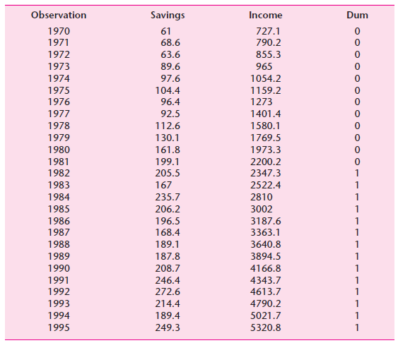
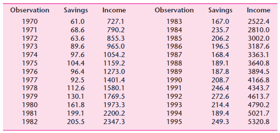
Use the data given in the following table and consider the following model:ln Savingsi = β1 + β2 ln Incomei + β3 ln Di + uiwhere ln stands for natural log and where Di = 1 for 1970€“1981 and 10 for 1982€“1995.a. What is the rationale behind
a. Show that if r1i = 0 for i = 2, 3, . . . , k then R1.23. . . k = 0b. What is the importance of this finding for the regression of variable X1(=Y) on X2, X3, . . . , Xk?
State with reason whether the following statements are true, false, or uncertain:a. Despite perfect multicollinearity, OLS estimators are BLUE.b. In cases of high multicollinearity, it is not possible to assess the individual significance of one or more partial regression coefficients.c. If an
Consider the following modelYi = α1 + α2Di + βXi + uiwhere Y = annual salary of a college professorX = years of teaching experienceD = dummy for genderConsider three ways of defining the dummy variable.a. D = 1 for male, 0 for female.b. D = 1 for female, 2 for male.c. D = 1 for female, −1 for
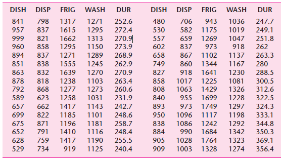
Refer to the quarterly appliance sales data given in the following table. Consider the following model:Salesi = α1 + α2D2i + α3D3i + α4D4i + uiwhere the D€™s are dummies taking 1 and 0 values for quarters II through IV.a. Estimate
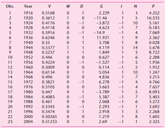
The following table 0gives data on quadrennial presidential elections in the United States from 1916 to 2004.*a. Using the data given in the following table, develop a suitable model to predict the Democratic share of the two-party presidential vote.b. How would you use this model to predict the
Refer to regression (9.6.4). Test the hypothesis that the rate of increase of average hourly earnings with respect to education differs by gender and race.
Refer to the regression (9.3.1). How would you modify the model to find out if there is any interaction between the gender and the region of residence dummies? Present the results based on this model and compare them with those given in Eq. (9.3.1).
Stepwise regression. In deciding on the “best” set of explanatory variables for a regression model, researchers often follow the method of stepwise regression. In this method one proceeds either by introducing the X variables one at a time (stepwise forward regression) or by including all the
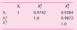
Refer to Example 7.4. For this problem the correlation matrix is as follows:a. €œSince the zero-order correlations are very high, there must be serious multicollinearity.€ Comment.b. Would you drop variables X2i and X3i from the model?c. If you drop them, what will happen to
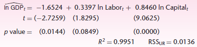
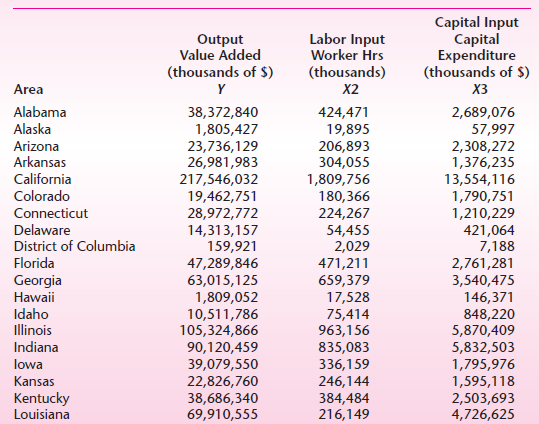
Refer to the illustrative example of Chapter 7 where we fitted the Cobb– Douglas production function to the manufacturing sector of all 50 states and the District of Columbia for 2005. The results of the regression given in Eq. (7.9.4) show that both the labor and capital coefficients are
Suppose in the modelYi = β1 + β2X2i + β3X3i + uithat r23, the coefficient of correlation between X2 and X3, is zero. Therefore, someone suggests that you run the following regressions:Yi = α1 + α2X2i + u1iYi = γ1 + γ3X3i + u2ia. Will α̂2 = β̂2 and γ̂3 = β̂3? Why?b. Will β̂1 equal
In data involving economic time series such as GNP, money supply, prices, income, unemployment, etc., multicollinearity is usually suspected. Why?
Consider the illustrative example of Section 10.6 (Example 10.1). How would you reconcile the difference in the marginal propensity to consume obtained from Eqs. (10.6.1) and (10.6.4)?
Consider the following model:Yt = β1 + β2Xt + β3Xt−1 + β4Xt−2 + β5Xt−3 + β6Xt−4 + utwhere Y = consumption, X = income, and t = time. The preceding model postulates that consumption expenditure at time t is a function not only of income at time t but also of income through previous
If the relation λ1X1i + λ2X2i + λ3X3i = 0 holds true for all values of λ1, λ2, and λ3, estimate r12.3, r13.2, and r23.1. Also find R21.23, R22.13, and R23.12. What is the degree of multicollinearity in this situation? Note: R21.23 is the coefficient of determination in the regression of Y on
In the model Yi = β1 + β2Di + ui , let Di = 0 for the first 40 observations and Di = 1 for the remaining 60 observations.You are told that ui has zero mean and a variance of 100. What are the mean values and variances of the two sets of observations?
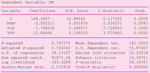
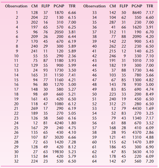
Refer to the child mortality example discussed in Chapter 8 (Example 8.1). The example there involved the regression of the child mortality (CM) rate on per capita GNP (PGNP) and female literacy rate (FLR). Now suppose we add the variable, total fertility rate (TFR). This gives the following
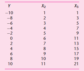
Consider the set of hypothetical data in the following table. Suppose you want to fit the modelYi = β1 + β2X2i + β3X3i + uito the data.a. Can you estimate the three unknowns? Why or why not?b. If not, what linear functions of these parameters, the estimable
In the k-variable linear regression model there are k normal equations to estimate the k unknowns. These normal equations are given in Appendix C. Assume that Xk is a perfect linear combination of the remaining X variables. How would you show that in this case it is impossible to estimate the k
Refer to the U.S. savings–income regression discussed in the chapter. As analternative to Eq. (9.5.1), consider the following model:ln Yt = β1 + β2Dt + β3Xt + β4(Dt Xt ) + utwhere Y is savings and X is income.a. Estimate the preceding model and compare the results with those given in Eq.
Refer to the Indian wage earners example (Section 9.12) and the data in Table 9.7.As a reminder, the variables are defined as follows:WI = weekly wage income in rupeesAge = age in yearsDsex = 1 for male workers and 0 for female workersDE2 = a dummy variable taking a value of 1 for workers with up
From annual data for 1972–1979, William Nordhaus estimated the following model to explain the OPEC’s oil price behavior (standard errors in parentheses).Ŷt = 0.3x1t + 5.22x2tse = (0.03) (0.50)wherey = difference between current and previous year’s price (dollars per barrel)x1
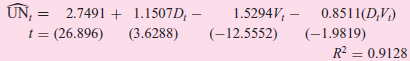
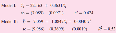
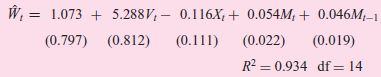
Consider the following regression results.* (The actual data are in the following table.)whereUN = unemployment rate, %V = job vacancy rate, %D = 1, for period beginning in 1966€“IV = 0, for period before 1966€“IVt = time, measured in quartersa. What are your prior
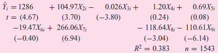
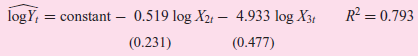
Consider the following regression results (t ratios are in parentheses):where Y = wife€™s annual desired hours of work, calculated as usual hours of work per year plus weeks looking for workX2 = after-tax real average hourly earnings of wifeX3 = husband€™s previous year
If you have monthly data over a number of years, how many dummy variables will you introduce to test the following hypotheses:a. All the 12 months of the year exhibit seasonal patterns.b. Only February, April, June, August, October, and December exhibit seasonal patterns.
Reconsider the savings–income regression in Section 8.7. Suppose we divide the sample into two periods as 1970–1982 and 1983–1995. Using the Chow test, decide if there is a structural change in the savings–income regression in the two periods. Comparing your results with those given in
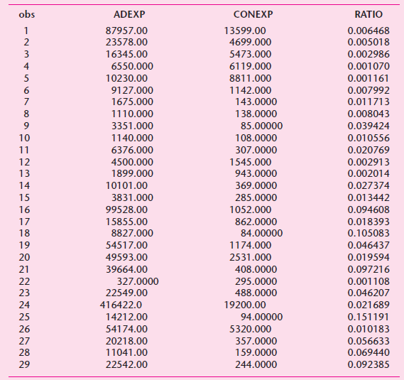
Return to Exercise 1.7, which gave data on advertising impressions retained and advertising expenditure for a sample of 21 firms. In Exercise 5.11 you were asked to plot these data and decide on an appropriate model about the relationship between impressions and advertising expenditure. Letting Y
Return to the child mortality example that we have discussed several times. In regression (7.6.2) we regressed child mortality (CM) on per capita GNP (PGNP) and female literacy rate (FLR). Now we extend this model by including total fertility rate (TFR). The data on all these variables are already
Refer to Example 8.3. Use the t test as shown in Eq. (8.6.4) to find out if there were constant returns to scale in the Mexican economy for the period of the study.In Example 8.3By way of illustrating the preceding discussion, consider the data given in the following table. Attempting to fit the
From annual data for the years 1968–1987, the following regression results were obtained:Ŷt = −859.92 + 0.6470X2t − 23.195X3t R2 = 0.9776 ……… (1)Ŷt = −261.09 + 0.2452X2t R2 = 0.9388 …….....................… (2)where Y = U.S. expenditure on imported goods, billions of 1982
Critical values of R2 when true R2 0. Equation (8.4.11) gave the relationship between F and R2 under the hypothesis that all partial slope coefficients are simultaneously equal to zero (i.e., R2 = 0). Just as we can find the critical F value at the α level of significance from the F table, we can
Refer to Exercise 7.21c. Now that you have the necessary tools, which test(s) would you use to choose between the two models? Show the necessary computations. (the dependent variables in the two models are different.)
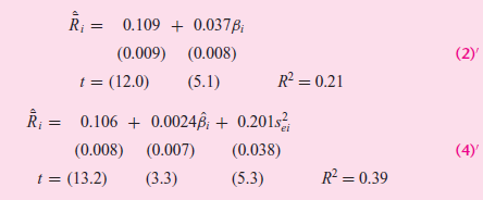
Estimating the capital asset pricing model (CAPM). In Section 6.1 we considered briefly the well-known capital asset pricing model of modern portfolio theory. In empirical analysis, the CAPM is estimated in two stages.Stage I (Time-series regression). For each of the N securities included in
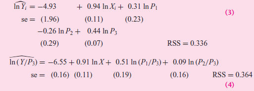
Marc Nerlove has estimated the following cost function for electricity generation:Y = AXβ Pα1 Pα2 Pα3u €¦€¦€¦€¦€¦.. (1)WhereY = total cost of productionX = output in kilowatt hoursP1 =
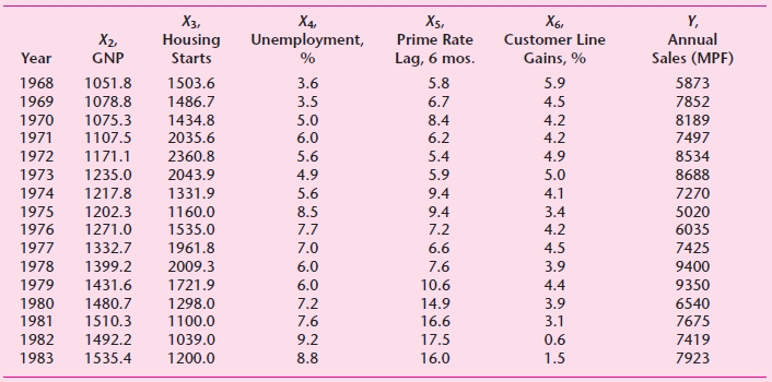
The demand for cable. The following table gives data used by a telephone cable manufacturer to predict sales to a major customer for the period 1968€“1983.The variables in the table are defined as follows:Y = annual sales in MPF, million paired feetX2 = gross national product (GNP), $,
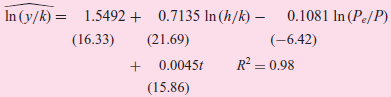
Consider the Cobb–Douglas production functionY = β1Lβ2Kβ3 ......................(1)where Y = output, L = labor input, and K = capital input. Dividing (1) through by K, we get(Y/K) = β1(L/K)β2Kβ2+β3−1 ......................(2)Taking the natural log of (2) and adding the error term, we
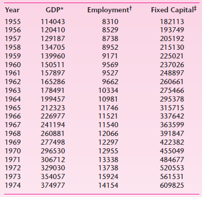
Energy prices and capital formation: United States, 1948€“1978. To test the hypothesis that a rise in the price of energy relative to output leads to a decline in the productivity of existing capital and labor resources, John A. Tatom estimated the following production function for the
The following is known as the transcendental production function (TPF), a generalization of the well-known Cobb€“Douglas production function:Yi = β1 Lβ2 kβ3 eβ4L+β5Kwhere Y = output, L = labor input, and K = capital input.After
Refer to the U.S. defense budget outlay regression estimated in Exercise 7.18.a. Comment generally on the estimated regression results.b. Set up the ANOVA table and test the hypothesis that all the partial slope coefficients are zero.
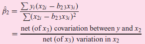
Refer to Exercise 7.17 relating to wildcat activity.a. Is each of the estimated slope coefficients individually statistically significant at the 5 percent level?b. Would you reject the hypothesis that R2 = 0?c. What is the instantaneous rate of growth of wildcat activity over the period
Refer to the demand for roses function of Exercise 7.16. Confining your considerations to the logarithmic specification,a. What is the estimated own-price elasticity of demand (i.e., elasticity with respect to the price of roses)?b. Is it statistically significant?c. If so, is it significantly
Show that F tests of Eq. (8.4.18) and Eq. (8.6.10) are equivalent.
Suppose you want to study the behavior of sales of a product, say, automobiles over a number of years and suppose someone suggests you try the following models:Yt = β0 + β1tYt = α0 + α1t + α2t2where Yt = sales at time t and t = time, measured in years. The first model postulates that sales is
From the Phillips curve given in Eq. (6.7.3), is it possible to estimate the natural rate of unemployment? How?
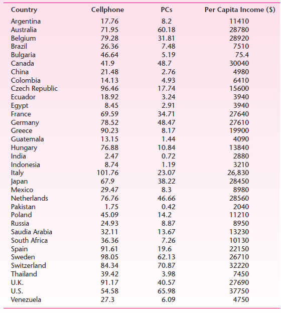
Refer to the data in the following table. To find out if people who own PCs also own cell phones, run the following regression:CellPhonei= β1+ β2PCsi+ uia. Estimate the parameters of this regression.b. Is the estimated slope coefficient statistically significant?c. Does it
Consider the following regression:SPIi = −17.8 + 33.2 Ginii se = (4.9) (11.8) r2= 0.16Where SPI = index of sociopolitical instability, average for 1960–1985, and Gini = Gini coefficient for 1975 or the closest available year within the range of
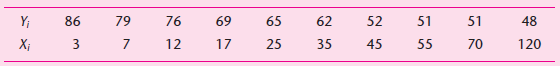
You are given the data in Table 6.7.**Fit the following model to these data and obtain the usual regression statistics and interpret the results:100 / (100 €“ Yi) = β1 + β2 (1/Xi) Y; X; 86 79 65 76 69 62 52 51 48 51 12 55 25 17 35 45 3 70 120
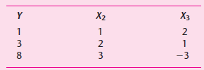
Consider the data in the following table.Based on these data, estimate the following regressions:Yi = α1 + α2X2i + u1i Yi = λ1 + λ3X3i + u2i Yi = β1 + β2X2i + β3X3i + ui Estimate only
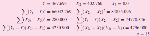
From the following data estimate the partial regression coefficients, their standard errors, and the adjusted and unadjusted R2values: Ỹ = 367.693 X2 = 402.760 X3 = 8.0 E(X2i – X2)² = 84855.096 (Y; – Ỹ)(X21 – X2) = 74778.346 E(X2i – X2)(X3i - X3) = 4796.000 EY, – Ý)? = 66042.269
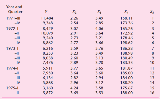
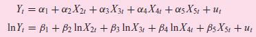
The demand for roses. The following table gives quarterly data on these variables:Y = quantity of roses sold, dozensX2= average wholesale price of roses, $/dozenX3= average wholesale price of carnations, $/dozenX4= average weekly family disposable income, $/weekX5= the trend variable taking values
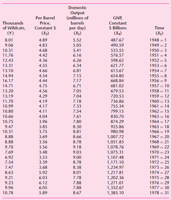
Wildcat activity. Wildcats are wells drilled to find and produce oil and/or gas in an improved area or to find a new reservoir in a field previously found to be productive of oil or gas or to extend the limit of a known oil or gas reservoir. The following gives data on these variables:Y = the
Show that Eq. (7.4.7) can also be expressed aswhere b23 is the slope coefficient in the regression of X2 on X3. Recall that b23 = Σx2ix3i / Σx23i. Ey,(x2 – b23x3i) E(x2; – b23x3)2 net (of x3) covariation between y and x2 net (of 3) variation in x2
In a multiple regression model you are told that the error term ui has the following probability distribution, namely, ui ∼ N(0, 4). How would you set up a Monte Carlo experiment to verify that the true variance is in fact 4?
Show that r212.3 = (R2 – r213 = (R2 – r213) / (1 – r213) and interpret the equation.
U.S. defense budget outlays, 1962€“1981. In order to explain the U.S. defense budget, you are asked to consider the following model:Yt = β1 + β2X2t + β3X3t + β4X4t + β5X5t + utwhereYt = defense budget-outlay for year t, $
If the relation α1X1 + α2X2 + α3X3 = 0 holds true for all values of X1, X2, and X3, find the values of the three partial correlation coefficients.
In a study of turnover in the labor market, James F. Ragan, Jr., obtained the following results for the U.S. economy for the period of 1950–I to 1979–IV.* (Figures in the parentheses are the estimated t statistics.)ln Ŷt = 4.47 – 0.34 lnX2t + 1.22 X2t + 1.22 ln X4t
The demand for chicken in the United States, 1960€“1982. To study the per capita consumption of chicken in the United States, you are given the data in the following table,where Y = per capita consumption of chickens, lbX2 = real disposable income per capita, $X3 = real retail price
Is it possible to obtain the following from a set of data?a. r23 = 0.9, r13 = −0.2, r12 = 0.8b. r12 = 0.6, r23 = −0.9, r31 = −0.5c. r21 = 0.01, r13 = 0.66, r23 = −0.7
Consider the following model:Yi = β1 + β2 Education i + β2 Years of experience + uiSuppose you leave out the years of experience variable. What kinds of problems or biases would you expect? Explain verbally.
Show that β2 and β3 in Eq. (7.9.2) do, in fact, give output elasticities of labor and capital.
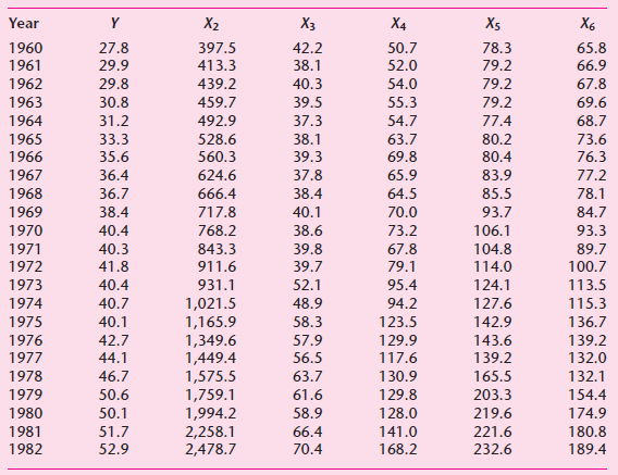
Consider the following demand function for money in the United States for the period 1980€“1998:Mt = β1 Yβ2t rβ3t eutwhere M = real money demand, using the M2 definition of moneyY = real GDPr = interest rateTo estimate the above demand for money
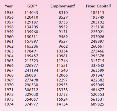
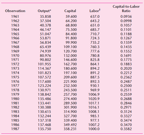
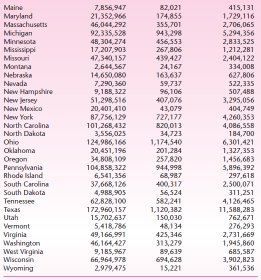
The following table gives data for the manufacturing sector of the Greek economy for the period 1961€“1987.a. See if the Cobb€“Douglas production function fits the data given in the table and interpret the results. What general conclusion do you draw?b. Now consider the
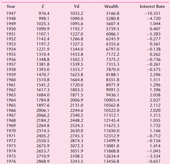
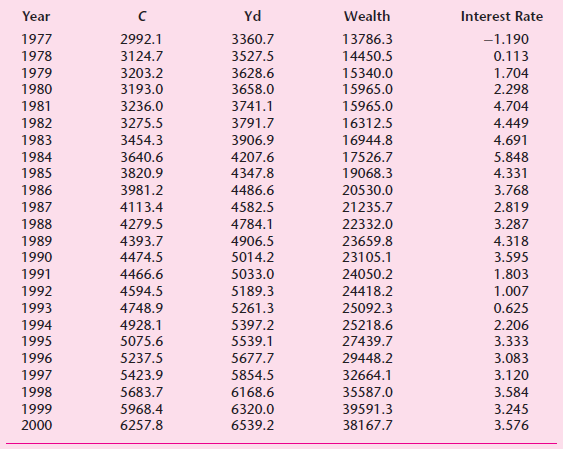
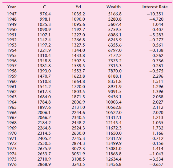
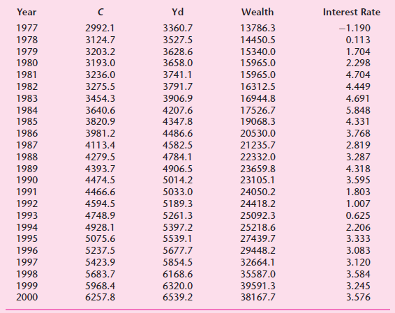
The following table gives data for real consumption expenditure, real income, real wealth, and real interest rates for the U.S. for the years 1947€“2000.a. Given the data in the table, estimate the linear consumption function using income, wealth, and interest rate. What is the fitted
In general R2≠ r212 + r213, but it is so only if r23 = 0. Comment and point out the significance of this finding.
Consider the following models.a. Will OLS estimates of α1 and β1 be the same? Why?b. Will OLS estimates of α3 and β3 be the same? Why?c. What is the relationship between α2 and β2?d. Can you compare the R2 terms of the
Suppose you estimate the consumption functionYi = α1 + α2Xi + u1iand the savings functionZi = β1 + β2Xi + u2iwhere Y = consumption, Z = savings, X = income, and X = Y + Z, that is, income is equal to consumption plus savings.a. What is the relationship, if any, between α2 and β2? Show your
Suppose you express the Cobb€“Douglas model given in Eq. (7.9.1) as follows:Yi = β1Xβ22i X β33i uiIf you take the log-transform of this model, you will have ln ui as the disturbance term on the right-hand side.a. What probabilistic assumptions do you
Regression through the origin. Consider the following regression through the origin:Yi = β̂2X2i + β̂3X3i + ûia. How would you go about estimating the unknowns?b. Will Σûi be zero for this model? Why or why not?c. Will Σûi X2i = Σûi X3i = 0 for this model?d. When would you use such a
Refer to Exercise 7.24 and the data in the following table concerning four economic variables in the U.S. from 1947€“2000.a. Based on the regression of consumption expenditure on real income, real wealth and real interest rate, find out which of the regression coefficients are
Suppose in the regressionln (Yi/X2i ) = α1 + α2 ln X2i + α3 ln X3i + uithe values of the regression coefficients and their standard errors are known. From this knowledge, how would you estimate the parameters and standard errors of the following regression model?ln Yi = β1 + β2 ln X2i + β3 ln
Refer to Section 8.8 and the data in the following table concerning disposable personal income and personal savings for the period 1970€“1995. In that section, the Chow test was introduced to see if a structural change occurred within the data between two time periods. Table 8.11 includes
Assume the following:Yi = β1 + β2X2i + β3X3i + β4X2i X3i + uiwhere Y is personal consumption expenditure, X2 is personal income, and X3 is personal wealth. The term (X2i X3i ) is known as the interaction term. What is meant by this expression? How would you test the hypothesis that the marginal
You are given the following regression results:Ŷt = 16,899 − 2978.5X2t R2 = 0.6149 t = (8.5152) (−4.7280)Ŷt = 9734.2 − 3782.2X2t
Based on our discussion of individual and joint tests of hypothesis based, respectively, on the t and F tests, which of the following situations are likely?1. Reject the joint null on the basis of the F statistic, but do not reject each separate null on the basis of the individual t tests.2. Reject
Refer to Exercise 7.21.a. What are the real income and interest rate elasticities of real cash balances?b. Are the preceding elasticities statistically significant individually?c. Test the overall significance of the estimated regression.d. Is the income elasticity of demand for real cash balances
From the data for 46 states in the United States for 1992, Baltagi obtained the following regression results:Log C = 4.30 – 1.24 log P + 0.17 log Y se = (0.91) (0.32) (0.20)
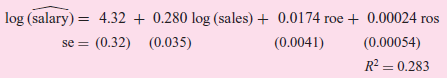
From a sample of 209 firms, Wooldridge obtained the following regression results:where salary = salary of CEOsales = annual firm salesroe = return on equity in percentros = return on firm€™s stockand where figures in the parentheses are the estimated standard errors.a. Interpret the
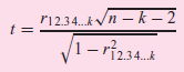
Assuming that Y and X2, X3, . . . , Xkare jointly normally distributed and assuming that the null hypothesis is that the population partial correlations are individually equal to zero, R. A. Fisher has shown thatfollows the t distribution with n ˆ’ k ˆ’ 2 df, where k is the
In studying the demand for farm tractors in the United States for the periods 1921€“1941 and 1948€“1957, Griliches€ obtained the following results:where Yt = value of stock of tractors on farms as of January 1, in 1935€“1939 dollars, X2 = index of prices
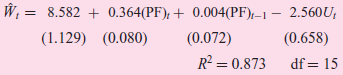
Consider the following wage-determination equation for the British economy* for the period 1950€“1969:whereW = wages and salaries per employeePF = prices of final output at factor costU = unemployment in Great Britain as a percentage of the total number of employees in Great Britaint =
A variation of the wage-determination equation given in Exercise 8.17 is as follows:whereW = wages and salaries per employeeV = unfilled job vacancies in Great Britain as a percentage of the total number of employees in Great BritainX = gross domestic product per person employedM = import
For the demand for chicken function estimated in Eq. (8.6.24), is the estimated income elasticity equal to 1? Is the price elasticity equal to −1?
For the demand function in Eq. (8.6.24) how would you test the hypothesis that the income elasticity is equal in value but opposite in sign to the price elasticity of demand? Show the necessary calculations. (cov [β̂2, β̂3] = −0.00142.)
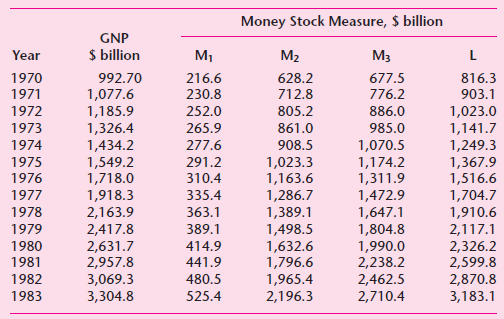
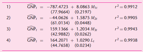
Table 5.6 gives data on GNP and four definitions of the money stock for the United States for 1970€“1983. Regressing GNP on the various definitions of money, we obtain the results shown in Table 5.7.Table 5.6Table 5.7The monetarists or quantity theorists maintain that nominal income
State with reason whether the following statements are true, false, or uncertain. Be precise.a. The t test of significance discussed in this chapter requires that the sampling distributions of estimators β̂1 and β̂2 follow the normal distribution.b. Even though the disturbance term in the CLRM
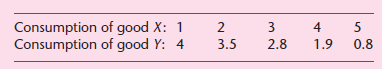
Suppose the equation of an indifference curve between two goods isXiYi= β1+ β2XiHow would you estimate the parameters of this model? Apply the preceding model to the data in the following table and comment on your results. Consumption of good X: 1 3 2.8 3.5 0.8 1.9
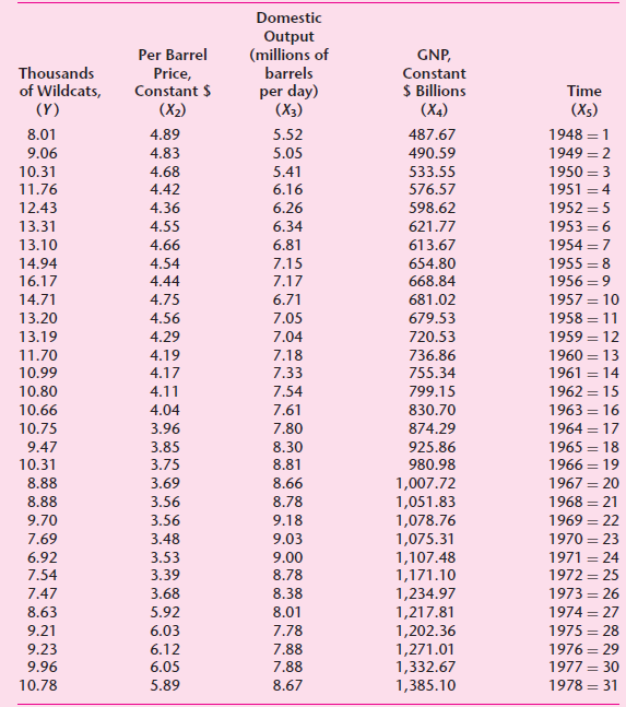
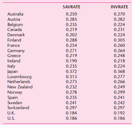
To study the relationship between investment rate (investment expenditure as a ratio of the GDP) and savings rate (savings as a ratio of GDP), Martin Feldstein and Charles Horioka obtained data for a sample of 21 countries. (See the following table.)The investment rate for each country is the
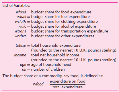
The following table gives the variable definitions for various kinds of expenditures, total expenditure, income, age of household, and the number of children for a sample of 1,519 households drawn from the 1980€“1982 British Family Expenditure Surveys.The actual dataset can be found on
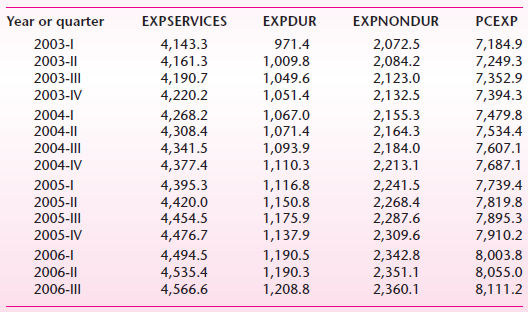
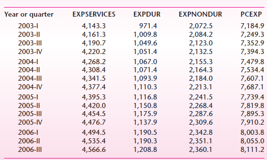
Refer to the following table. Find out the rate of growth of expenditure on durable goods. What is the estimated semielasticity? Interpret your results. Would it make sense to run a double log regression with expenditure on durable goods as the regress and and time as the regress or? How would you
From the data given in the following table, find out the growth rate of expenditure on nondurable goods and compare your results with those obtained from Exercise 6.17. PCEXP Year or quarter EXPSERVICES EXPDUR EXPNONDUR 4,143.3 4,161.3 4,190.7 4,220.2 7,184.9 7,249.3 7,352.9 7,394.3 2003-1 971.4
Consider the regression modelyi = β1 + β2xi + uiwhere yi = (Yi – Y̅ ) and xi = (Xi – X̅ ). In this case, the regression line must pass through the origin. True or false? Show your calculations.
Consider the log–linear model:ln Yi = β1 + β2 ln Xi + uiPlot Y on the vertical axis and X on the horizontal axis. Draw the curves showing the relationship between Y and X when β2 = 1, and when β2 > 1, and when β2 < 1.
The following table gives data for the U.K. on total consumer expenditure (in £ millions) and advertising expenditure (in £ millions) for 29 product categories.a. Considering the various functional forms we have discussed in the chapter, which functional form might fit the data given in
The following regression results were based on monthly data over the period January 1978 to December 1987:Ŷt = 0.00681 ................... + 0.75815Xtse = (0.02596) .................. (0.27009)t = (0.26229) ..................... (2.80700)p value = (0.7984) .............(0.0186) r2 = 0.4406Ŷt =
Consider the following models:Model I: Yi = β1 + β2Xi + uiModel II: Y*i α1 + α2X∗i + uiwhere Y* and X* are standardized variables. Show that α̂2 = β̂2(Sx/Sy ) and hence establish that although the regression slope coefficients are independent of the change of origin they are not
Consider the following regression model:1/Yi = β1 + β2 (1/Xi) + uiNeither Y nor X assumes zero value.a. Is this a linear regression model?b. How would you estimate this model?c. What is the behavior of Y as X tends to infinity?d. Can you give an example where such a model may be appropriate?
Consider the following models:ln Y∗i = α1 + α2 ln X∗i + u∗iln Yi = β1 + β2 ln Xi + uiwhere Y∗i = w1Yi and X∗i = w2Xi , the w’s being constants.a. Establish the relationships between the two sets of regression coefficients and their standard errors.b. Is the r2 different between the
Showing 3900 - 4000
of 4105
First
28
29
30
31
32
33
34
35
36
37
38
39
40
41
42
Step by Step Answers