New Semester
Started
Get
50% OFF
Study Help!
--h --m --s
Claim Now
Question Answers
Textbooks
Find textbooks, questions and answers
Oops, something went wrong!
Change your search query and then try again
S
Books
FREE
Study Help
Expert Questions
Accounting
General Management
Mathematics
Finance
Organizational Behaviour
Law
Physics
Operating System
Management Leadership
Sociology
Programming
Marketing
Database
Computer Network
Economics
Textbooks Solutions
Accounting
Managerial Accounting
Management Leadership
Cost Accounting
Statistics
Business Law
Corporate Finance
Finance
Economics
Auditing
Tutors
Online Tutors
Find a Tutor
Hire a Tutor
Become a Tutor
AI Tutor
AI Study Planner
NEW
Sell Books
Search
Search
Sign In
Register
study help
business
econometrics
Basic Econometrics 5th edition Damodar N. Gujrati, Dawn C. Porter - Solutions
Develop a simultaneous-equation model for the supply of and demand for dentists in the United States. Specify the endogenous and exogenous variables in the model.
Develop a simple model of the demand for and supply of money in the United States and compare your model with those developed by K. Brunner and A. H. Meltzer* and R. Tiegen.
a. For the demand-and-supply model of Example 18.1, obtain the expression for the probability limit of α̂1.b. Under what conditions will this probability limit be equal to the true α1?
For the IS-LM model discussed in the text, find the level of interest rate and income that is simultaneously compatible with the goods and money market equilibrium.
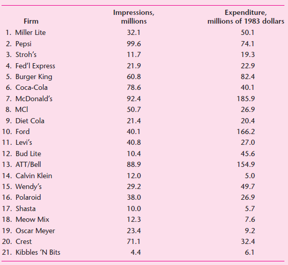
To study the relationship between inflation and yield on common stock, Bruno Oudet€¡ used the following model:where L = real per capita monetary baseY = real per capita incomeI = the expected rate of inflationNIS = a new issue variableE = expected end-of-period stock returns, proxied by
In their article, €œA Model of the Distribution of Branded Personal Products in Jamaica,€™€™* John U. Farley and Harold J. Levitt developed the following model (the personal products considered were shaving cream, skin cream, sanitary napkins, and toothpaste):WhereY1 =
To study the relationship between advertising expenditure and sales of cigarettes, Frank Bass used the following model:WhereY1 = logarithm of sales of filter cigarettes (number of cigarettes) divided by population over age 20Y2 = logarithm of sales of nonfilter cigarettes (number of cigarettes)
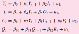
G. Menges developed the following econometric model for the West German economy:where Y = national incomeI = net capital formationC = personal consumptionQ = profitsP = cost of living indexR = industrial productivityt = timeu = stochastic disturbancesa. Which of the variables would you regard as
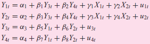
L. E. Gallaway and P. E. Smith developed a simple model for the United States economy, which is as follows:Y = gross national productC = personal consumption expenditureI = gross private domestic investmentG = government expenditure plus net foreign investmentYD = disposable, or after-tax, incomeM
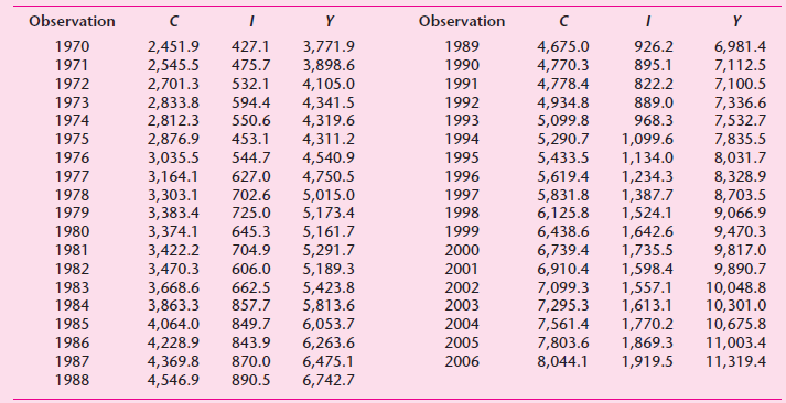
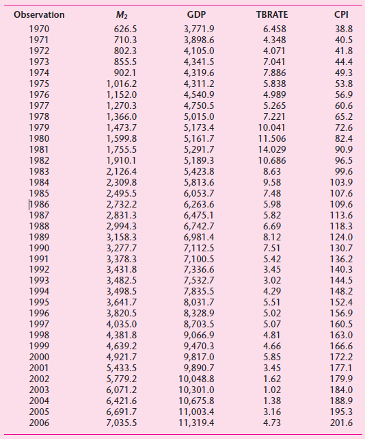
The following table gives you data on Y (gross domestic product), I (gross private domestic investment), and C (personal consumption expenditure) for the United States for the period 1970€“2006. All data are in 1996 billions of dollars. Assume that C is linearly related to Y as in the
Using the data given in Exercise 18.10, regress gross domestic investment I on GDP and save the results for further examination in a later chapter.
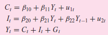
Consider the macroeconomics identityC + I = Y ( = GDP)As before, assume thatCt = β0 + β1Yt + utand, following the accelerator model of macroeconomics, letIt = α0 + α1(Yt − Yt−1) + vtwhere u and v are error terms. From the data given in Exercise 18.10, estimate the accelerator model and save
Supply and demand for gas. Table 18.3, found on the textbook website, gives data on some of the variables that determine demand for and supply of gasoline in the U.S. from January 1978 to August 2002.* The variables are: pricegas (cents per gallon); quantgas (thousands of barrels per day,
Show that the two definitions of the order condition of identification (see Section 19.3) are equivalent.
Deduce the structural coefficients from the reduced-form coefficients given in Eqs. (19.2.25) and (19.2.27).
Obtain the reduced form of the following models and determine in each case whether the structural equations are unidentified, just identified, or over identified:a. Chap. 18, Example 18.2.b. Chap. 18, Example 18.3.c. Chap. 18, Example 18.6.
In the model (19.2.22) of the text it was shown that the supply equation was over identified. What restrictions, if any, on the structural parameters will make this equation just identified? Justify the restrictions you impose.
From the modelthe following reduced-form equations are obtained:a. Are the structural equations identified?b. What happens to identification if it is known a priori that γ11 = 0? Y1 = B10 + B12 Y2ı + Y11X1 +u11 Yu = B20 + B21 Y1u + Y22X21 + u21 Yu = l10 + M11X11 + 112X21 + W; Y2 = l20
Refer to Exercise 19.6. The estimated reduced-form equations are as follows:Y1t = 4 + 3X1t + 8X2tY2t = 2 + 6X1t + 10X2ta. Obtain the values of the structural parameters.b. How would you test the null hypothesis that γ11 = 0?
The modelproduces the following reduced-form equations:Y1t = 4 + 8X1tY2t = 2 + 12X1ta. Which structural coefficients, if any, can be estimated from the reduced-form coefficients? Demonstrate your contention.b. How does the answer to (a) change if it is known a priori that (1) β12 = 0
Determine whether the structural equations of the model given in Exercise 18.8 are identified.
Refer to Exercise 18.7 and find out which structural equations can be identified.
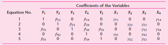
The following table is a model in five equations with five endogenous variables Y and four exogenous variables X:Determine the identifiability of each equation with the aid of the order and rank conditions of identifications. Coefficients of the Variables Y3 Y4 Equation No. X1 Y1 Y2 Ys X2 X3 X4 Y14
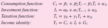
Consider the following extended Keynesian model of income determination:WhereC = consumption expenditureY = incomeI = investmentT = taxesG = government expenditureu€™s = the disturbance termsIn the model the endogenous variables are C, I, T, andY and the predetermined variables are G and
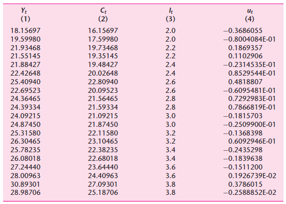
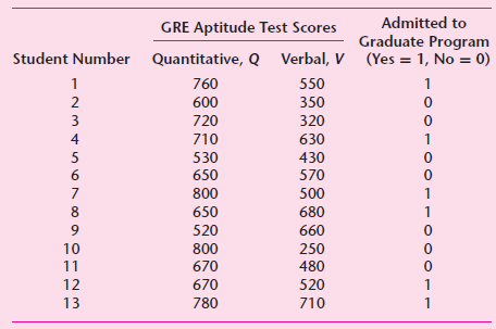
Refer to the data given in the following table of Chapter 18. Using these data, estimate the reduced-form regressions (19.1.2) and (19.1.4). Can you estimate β0and β1? Show your calculations. Is the model identified? Why or why not? Y: (1) Ut (2) (3) (4) 2.0 -0.3686055
Suppose we propose yet another definition of the order condition of identifiability:K ≥ m + k − 1which states that the number of predetermined variables in the system can be no less than the number of unknown coefficients in the equation to be identified. Show that this definition is equivalent
A simplified version of Suits€™s model of the watermelon market is as follows:*WhereP = price(Q/N) = per capita quantity demanded(Y/N) = per capita incomeFt = freight costs(P/W) = price relative to the farm wage rateC = price of cottonT = price of other vegetablesN = populationP and Q are
Consider the following demand-and-supply model for money:Money demand: Mdt = β0 + β1Yt + β2Rt + β3Pt + u1tMoney supply: Mst = α0 + α1Yt + u2tWhereM =moneyY = incomeR = rate of interestP =priceu€™s = error
The Hausman test discussed in the text can also be conducted in the following way. Consider Eq. (19.4.7):Qt = β0 + β1Pt + β1vt + u2ta. Since Pt and vt have the same coefficients, how would you test that in a given application that is indeed the case? What are the implications of this?b. Since Pt
State whether each of the following statements is true or false:a. The method of OLS is not applicable to estimate a structural equation in a simultaneous equation model.b. In case an equation is not identified, 2SLS is not applicable.c. The problem of simultaneity does not arise in a recursive
Why is it unnecessary to apply the two-stage least-squares method to exactly identified equations?
Consider the following modified Keynesian model of income determination:where C = consumption expenditureI = investment expenditureY = incomeG = government expenditureGt and Ytˆ’1 are assumed predetermineda. Obtain the reduced-form equations and determine which of the preceding equations
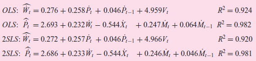
Consider the following results:where WÌ‚t , PÌ‚t , MÌ‚t , and XÌ‚t are percentage changes in earnings, prices, import prices, and labor productivity (all percentage changes are over the previous year), respectively, and where Vt represents
Assume that production is characterized by the Cobb€“Douglas production functionQi = AKαi LβiWhereQ = outputK = capital inputL = labor inputA, α, and β = parametersi = ith firmGiven the price of final output P, the price of labor W, and
Consider the following demand-and-supply model for money:WhereM = moneyY = incomeR = rate of interestP = priceAssume that R and P are predetermined.a. Is the demand function identified?b. Is the supply function identified?c. Which method would you use to estimate the parameters of the identified
Refer to Exercise 18.10. For the two-equation system there obtain the reduced-form equations and estimate their parameters. Estimate the indirect least-squares regression of consumption on income and compare your results with the OLS regression.
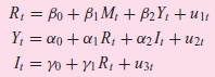
Consider the following model:Rt = β0 + β1Mt + β2Yt + u1tYt = α0 + α1Rt + u2twhere Mt (money supply) is exogenous, Rt is the interest rate, and Yt is GDP.a. How would you justify the model?b. Are the equations identified?c. Using the
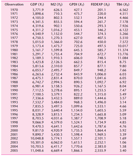
Suppose we change the model in Exercise 20.8 as follows:Rt = β0 + β1Mt + β2Yt + β3Ytˆ’1 + u1tYt = α0 + α1Rt + u2ta. Find out if the system is identified.b. Using the data given in the following table, estimate the
Consider the following model:Rt = β0 + β1Mt + β2Yt + u1tYt = α0 + α1Rt + α2 It + u2twhere the variables are as defined in Exercise 20.8. Treating I (domestic investment) and M exogenously, determine the identification of
Suppose we change the model of Exercise 20.10 as follows:Assume that M is determined exogenously.a. Find out which of the equations are identified.b. Estimate the parameters of the identified equation(s) using the data given in the following table. Justify your method(s). R; = Bo + B1 M; + B2Y1
Verify the standard errors reported in Eq. (20.5.3).
Return to the demand-and-supply model given in Eqs. (20.3.1) and (20.3.2).Suppose the supply function is altered as follows:Qt = β0 + β1Ptˆ’1 + u2twhere Ptˆ’1 is the price prevailing in the previous period.a. If X (expenditure) and Ptˆ’1 are
In this exercise we examine data for 534 workers obtained from the Current Population Survey (CPS) for 1985. The data can be found as Table 20.10 on the textbook website. The variables in this table are defined as follows:W = wages $, per hour; occup = occupation; sector = 1 for manufacturing, 2
Explain with a brief reason whether the following statements are true, false, or uncertain:a. All econometric models are essentially dynamic.b. The Koyck model will not make much sense if some of the distributed-lag coefficients are positive and some are negative.c. If the Koyck and adaptive
Prove Eq. (17.8.3).cov [Yt−1, (ut − λut−1)] = −λσ2 17.8.3
Assume that prices are formed according to the following adaptive expectations hypothesis:where P* is the expected price and P the actual price. Complete the following table, assuming γ = 0.5:* P: = y P,-1 +(1 –v)P, Period p* 100 110 125 155 185 t+1
Consider the modelSuppose Ytˆ’1 and vt are correlated. To remove the correlation, suppose we use the following instrumental variable approach: First regress Yt on X1t and X2t and obtain the estimated YÌ‚t from this regression. Then regresswhere YÌ‚tˆ’1
a. Evaluate the median lag for λ = 0.2, 0.4, 0.6, 0.8.b. Is there any systematic relationship between the value of λ and the value of the median lag?
a. Prove that for the Koyck model, the mean lag is as shown in Eq. (17.4.10).b. If λ is relatively large, what are its implications?
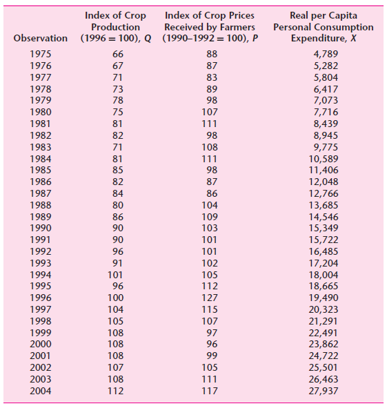
Using the formula for the mean lag given in Eq. (17.4.9), verify the mean lag of 10.959 quarters reported in the illustration of the following table. Coeff. Coeff. Coeff. It| 3.249 3.783 |t| It| 3.943 3.712 3.511 3.338 3.191 7.870 5.634 0.048 mg 0.054 mg 0.059 4.305 0.069 0.062 0.053 0.039
Supposewhere M = demand for real cash balances, Y* = expected real income, and R* = expected interest rate. Assume that expectations are formulated as follows:where γ1 and γ2 are coefficients of expectation, both lying between 0 and 1.a. How would you express Mt in terms of
If you estimate Eq. (17.7.2) by OLS, can you derive estimates of the original parameters? What problems do you foresee? (For details, see Roger N. Waud.)
Consider the following model:Yt = α + βXt + utAssume that ut follows the Markov first-order autoregressive scheme given in Chapter 12, namely,ut = put-1 + εtwhere Ï is the coefficient of (first-order) autocorrelation and where εt
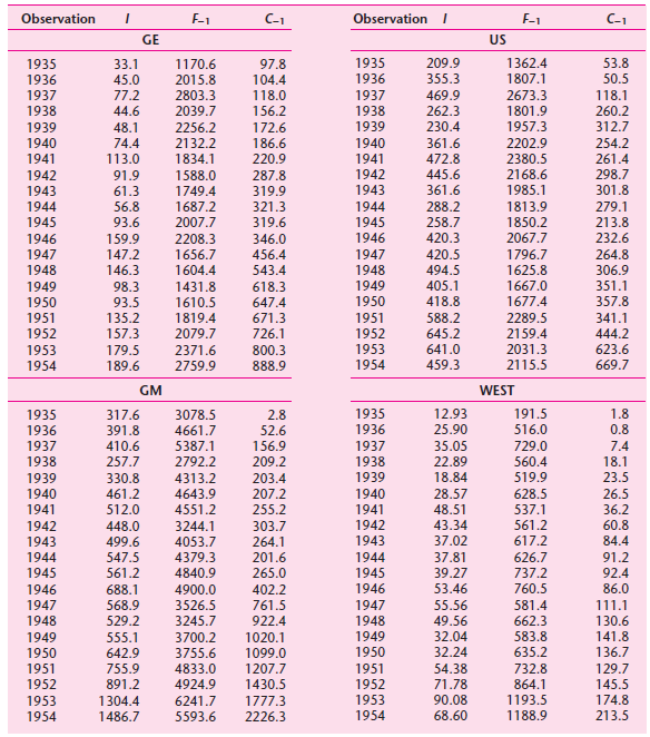
Use the investment data given in the following table.a. Estimate the Grunfeld investment function for each company individually.b. Now pool the data for all the companies and estimate the Grunfeld investment function by OLS.c. Use LSDV to estimate the investment function and compare your results
Refer to the data in the following table.a. Let Y = eggs produced (in millions) and X = price of eggs (cents per dozen). Estimate the model for the years 1990 and 1991 separately.b. Pool the observations for the two years and estimate the pooled regression. What assumptions are you making in
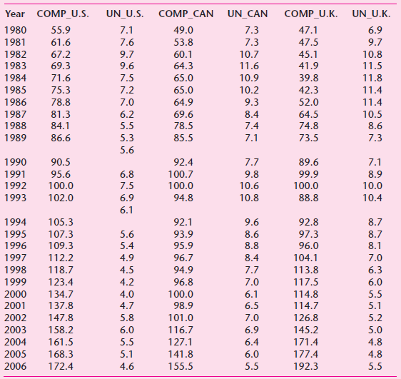
Refer to the airline example discussed in the text. Instead of the linear model given in Eq. (16.4.2), estimate a log€“linear regression model and compare your results with those given in the following table. Year COMP_U.S. UN_U.S. COMP_CAN UN_CAN COMP_U.K. UN_U.K. 1980 55.9 7.1 49.0 7.3
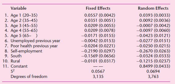
Based on the Michigan Income Dynamics Study, Hausman attempted to estimate a wage, or earnings, model using a sample of 629 high school graduates, who were followed for a period of six years, thus giving in all 3,774 observations. The dependent variable in this study was logarithm of wage, and the
For the investment data given in the following table, which model would you choose€”FEM or REM? Why? C-1 C-1 F-1 Observation E-1 Observation GE US 1935 1935 209.9 1362.4 53.8 33.1 1170.6 97.8 45.0 77.2 1936 355.3 1807.1 50.5 1936 2015.8 104.4 1937 1938 1939 1940 1941 2803.3 118.0 1937
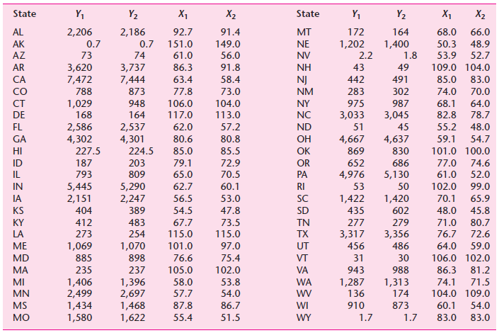
Refer to the data on eggs produced and their prices given in the following table. Which model may be appropriate here, FEM or ECM? Why? State Y1 Y2 X1 X2 State Y, Y2 X1 X2 92.7 66.0 AL 2,206 2,186 91.4 мT 172 164 68.0 149.0 1,202 1,400 AK 0.7 0.7 151.0 NE 50.3 48.9 AZ 73 74 61.0 56.0 NV 2.2 1.8
How would you extend model (16.4.2) to allow for a time error component? Write down the model explicitly.
When are panel data regression models inappropriate? Give examples.
Is there a difference between LSDV, within-estimator, and first-difference models?
What is meant by an error components model (ECM)? How does it differ from FEM? When is ECM appropriate? And when is FEM appropriate?
What is meant by a fixed effects model (FEM)? Since panel data have both time and space dimensions, how does FEM allow for both dimensions?
What are the special features of (a) cross-section data, (b) time series data, and (c) panel data?
Download the data set Benign, which is Table 15.29, from the textbook website. The variable cancer is a dummy variable, where 1 = had breast cancer and 0 = did not have breast cancer.* Using the variables age (= age of subject), HIGD (= highest grade completed in school), CHK (= 0 if subject did
For the smokers example discussed in the text (see Section 15.10) download the data from the textbook website in Table 15.28. See if the product of education and income (i.e., the interaction effect) has any effect on the probability of becoming a smoker.
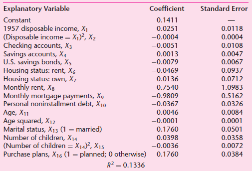
Table 15.27 on the textbook website gives data for 2,000 women regarding work (1 = a woman works, 0 = otherwise), age, marital status (1 = married, 0 = otherwise), number of children, and education (number of years of schooling). Out of a total of 2,000 women, 657 were recorded as not being wage
Monte Carlo study. As an aid to understanding the probit model, William Becker and Donald Waldman assumed the following:E(Y | X) = ˆ’1 + 3XThen, letting Yi = ˆ’1 + 3X + εi , where εi is assumed standard normal (i.e., zero mean and unit variance), they
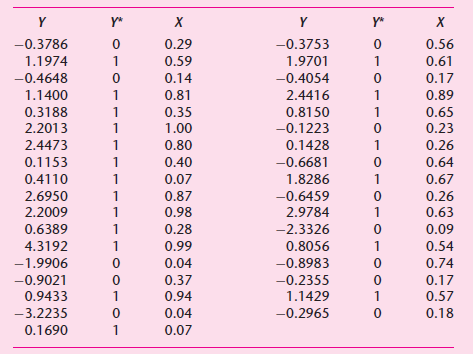
To find out who has a bank account (checking, savings, etc.) and who doesn€™t, John Caskey and Andrew Peterson estimated a probit model for the years 1977 and 1989, using data on U.S. households. The results are given in Table 15.25. The values of the slope coefficients given in the table
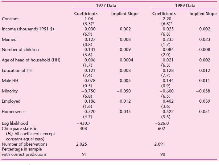
To study the effectiveness of a price discount coupon on a six-pack of a soft drink, Douglas Montgomery and Elizabeth Peck collected the data shown in the following table. A sample of 5,500 consumers was randomly assigned to the eleven discount categories shown in the table, 500 per category. The
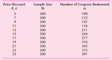
Thirteen applicants to a graduate program had quantitative and verbal scores on the GRE as listed in the following table. Six students were admitted to the program.a. Use the LPM to predict the probability of admission to the program based on quantitative and verbal scores in the GRE.b. Is this a
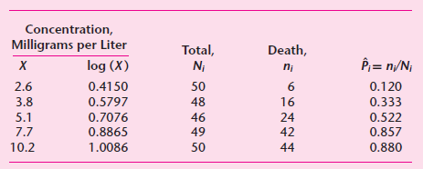
The following table gives data on the results of spraying rotenone of different concentrations on the chrysanthemum aphis in batches of approximately fifty. Develop a suitable model to express the probability of death as a function of the log of X, the log of dosage, and comment on the results.
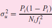
In the probit model given in the following table the disturbance ui has this variance:where fi is the standard normal density function evaluated at Fˆ’1(Pi).a. Given the preceding variance of ui, how would you transform the model in Table 15.10 to make the resulting error term
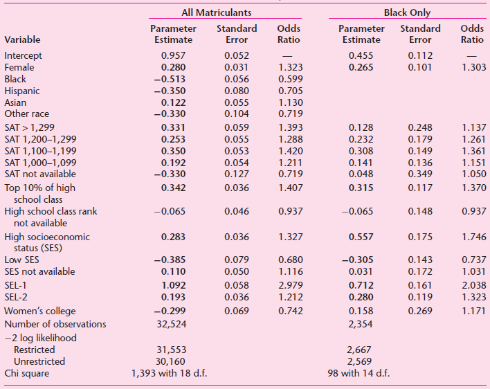
In an important study of college graduation rates of all high school matriculants and Black-only matriculants, Bowen and Bok obtained the results in the following table, based on the logit model.*a. What general conclusion do you draw about graduation rates of all matriculants and black only
From the household budget survey of 1980 of the Dutch Central Bureau of Statistics, J. S. Cramer obtained the following logit model based on a sample of 2,820 households. (The results given here are based on the method of maximum likelihood and are after the third iteration.) The purpose of the
Compare and comment on the OLS and WLS regressions in Eqs. (15.7.3) and (15.7.1).
From data for 54 standard metropolitan statistical areas (SMSA), Demaris estimated the following logit model to explain high murder rate versus low murder rate:**ln Ôi = 1.1387 + 0.0014Pi + 0.0561Ci − 0.4050Rise = (0.0009) (0.0227) (0.1568)where O = the odds of a high murder rate, P = 1980
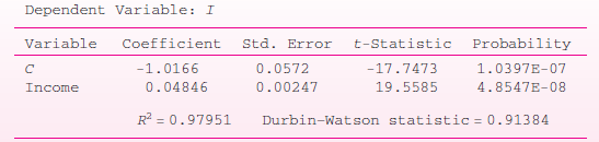
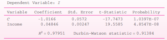
In the probit regression given in the following table show that the intercept is equal to ˆ’μx/σxand the slope is equal to 1/σx, where μxand σxare the mean and standard deviation of X. Dependent Variable: I Coefficient Variable
Estimate the probabilities of owning a house at the various income levels underlying the regression (15.7.1). Plot them against income and comment on the resulting relationship.
In studying the purchase of durable goods Y (Y = 1 if purchased, Y = 0 if no purchase) as a function of several variables for a total of 762 households, Janet A. Fisherˆ—obtained the following LPM results:a. Comment generally on the fit of the equation.b. How would you interpret the
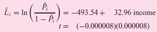
For the home ownership data given in Table 15.1, the maximum likelihood estimates of the logit model are as follows:Comment on these results, bearing in mind that all values of income above 16 (thousand dollars) correspond to Y = 1 and all values of income below 16 correspond to Y = 0. A priori,
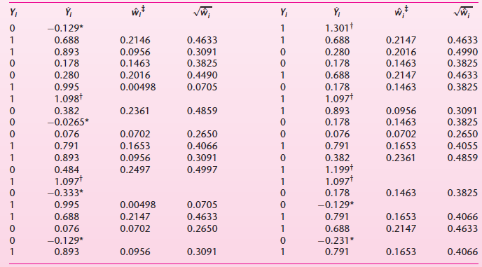
Refer to the data given in the following table. If YÌ‚iis negative, assume it to be equal to 0.01 and if it is greater than 1, assume it to be equal to 0.99. Recalculate the weights wiand estimate the LPM using WLS. Compare your results with those given in Eq. (15.2.11) and comment. Y;
The following table gives data on real GDP, labor, and capital for Mexico for the period 1955€“1974. See if the multiplicative Cobb€“Douglas production function given in Eq. (14.1.2a) fits these data. Compare your results with those obtained from fitting the additive
Show that βˆ—2of Eq. (11.3.8) can also be expressed asand var (βˆ—2) given in Eq. (11.3.9) can also be expressed aswhere yˆ—i = Yi €“ YÌ…ˆ— and xˆ—i = Xi €“ XÌ…ˆ—
Evaluate the following statement made by Henry Theil:Given the present state of the art, the most sensible procedure is to interpret confidence coefficients and significance limits liberally when confidence intervals and test statistics are computed from the final regression of a regression
Commenting on the econometric methodology practiced in the 1950s and early 1960s, Blaug stated:. . . much of it [i.e., empirical research] is like playing tennis with the net down:instead of attempting to refute testable predictions, modern economists all too frequently are satisfied to demonstrate
According to Blaug, “There is no logic of proof but there is logic of disproof.” What does he mean by this?
Refer to the St. Louis model discussed in the text. Keeping in mind the problems associated with the nested F test, critically evaluate the results presented in regression (13.8.4).
Suppose the true model isYi = β1 + β2Xi + βX2i + β3X3i + uiBut you estimateYi = α1 + α2Xi + viIf you use observations of Y at X = −3, −2, −1, 0, 1, 2, 3, and estimate the “incorrect” model, what bias will result in these estimates?
To see if the variable X2i belongs in the model Yi = β1 + β2Xi + ui , Ramsey’s RESET test would estimate the linear model, obtaining the estimated Yi values from this model [i.e., Ŷi = β̂1 + β̂2Xi ] and then estimating the model Yi = α1 + α2Xi+ α3Ŷ2i+ vi and testing the significance
Use the data for the demand for chicken given in Exercise 7.19. Suppose you are told that the true demand function isln Yt = β1 + β2 ln X2t + β3 ln X3t + β6 ln X6t + ut ……………… (1)but you think differently and estimate the following demand function:ln Yt = α1 + α2 ln X2t + α3 ln
Continue with Exercise 13.21. Strictly for pedagogical purposes, assume that model (2) is the true demand function.a. If we now estimate model (1), what type of specification error is committed in this instance?b. What are the theoretical consequences of this specification error? Illustrate with
Monte Carlo experiment.* Ten individuals had weekly permanent income as follows:$200, 220, 240, 260, 280, 300, 320, 340, 380, and 400. Permanent consumption (Y∗i) was related to permanent income X∗i asY∗i = 0.8X∗i …………… (1)Each of these individuals had transitory income equal to
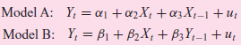
Continue with Exercise 13.25. Using the J test, how would you decide between the two models?Data from 13.25Refer to Exercise 8.26. With the definitions of the variables given there, consider the following two models to explain Y:Model A: Yt = α1 + α2X3t + α3X4t + α4X6t + utModel B: Yt = β1 +
Refer to Exercise 7.19, which is concerned with the demand for chicken in the United States. There you were given five models.a. What is the difference between model 1 and model 2? If model 2 is correct and you estimate model 1, what kind of error is committed? Which test would you apply—equation
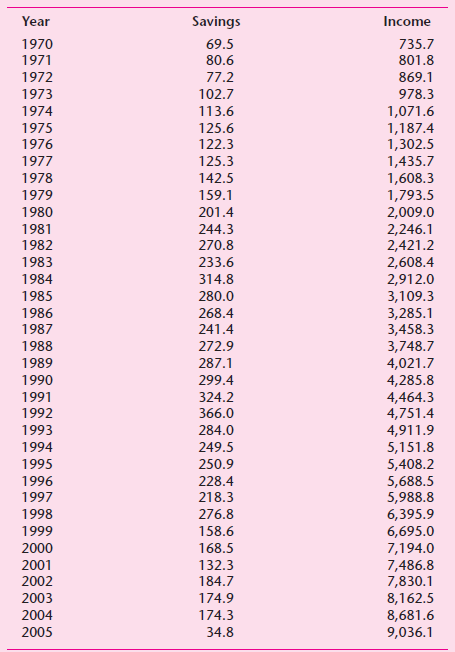
Refer to the following table, which gives data on personal savings (Y) and personal disposable income (X) for the period 1970€“2005. Now consider the following models:How would you choose between these two models? State clearly the test procedure(s) you use and show all the calculations.
Use the data in Exercise 13.28.To familiarize yourself with recursive least squares, estimate the savings functions for 1970€“1981, 1970€“1985, 1970€“1990, and 1970€“1995. Comment on the stability of estimated coefficients in the savings functions.Data from
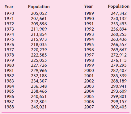
The data in the following table gives U.S. population, in millions of persons, for the period 1970€“2007. Fit the growth models given in Exercise 14.7 and decide which model gives a better fit. Interpret the parameters of the model. Population Year Population Year 205,052 207,661 209,896
Continue with Exercise 13.29, but now use the updated data in Table 8.10.a. Suppose you estimate the savings function for 1970–1981. Using the parameters thus estimated and the personal disposable income data from 1982–2000, estimate the predicted savings for the latter period and use Chow’s
Showing 3700 - 3800
of 4105
First
28
29
30
31
32
33
34
35
36
37
38
39
40
41
42
Step by Step Answers
![Rht αι + α R + α3Rhr-1 + αL, + as + αςNIS, + α7] +ur RΒ +β) RH+ βRb,-1 + β,L+ β5Y+ β6NIS, + βΕ+ Lλ st](https://dsd5zvtm8ll6.cloudfront.net/si.question.images/images/question_images/1525/4/3/8/4385aec57e6d190c1525438423899.jpg)
![|Yli = a1 + B1 Y2i + B2Y3¡ + B3Y4¡ + U ]i | Y2i = a2 + B4Y1; + B3 Ysi + yı X1i + y2X2i + u2i Y3i = a3 + B6 Y2i + Y3X3](https://dsd5zvtm8ll6.cloudfront.net/si.question.images/images/question_images/1525/4/3/8/4935aec581d9d2e31525438480954.jpg)
![Y; = C, + I; + G; C; = B1 + B2YD,–1+ B3M, + u]; I, = B4 + Bs(Y,-1 – Y;-2) + B6Z¡–1 + u2: G = B7 + BsG,-1+U31](https://dsd5zvtm8ll6.cloudfront.net/si.question.images/images/question_images/1525/4/3/8/6015aec5889c8e2a1525438588249.jpg)