All Matches
Solution Library
Expert Answer
Textbooks
Search Textbook questions, tutors and Books
Oops, something went wrong!
Change your search query and then try again
Toggle navigation
FREE Trial
S
Books
FREE
Tutors
Study Help
Expert Questions
Accounting
General Management
Mathematics
Finance
Organizational Behaviour
Law
Physics
Operating System
Management Leadership
Sociology
Programming
Marketing
Database
Computer Network
Economics
Textbooks Solutions
Accounting
Managerial Accounting
Management Leadership
Cost Accounting
Statistics
Business Law
Corporate Finance
Finance
Economics
Auditing
Ask a Question
Search
Search
Sign In
Register
study help
business
financial modeling
Questions and Answers of
Financial Modeling
An ill-conditioned matrix is a matrix that ?almost doesn?t have? an inverse. A set of examples of such matrices are Hilbert matrices. An n-dimensional Hilbert matrix looks like: a. Calculate the
Solve the equations AX = Y, where: [ 13 -8 -3] Г20 X1 А3D|-8 10 -1|, Ү %3D| -5|, X-| x, [-3 -1 11] X3
Solve the following system of equations by using matrices: Зх +4у -62 -9w%3D15 2.x 2х -у +w =2 y +7 +w=3 +y = 1
Transpose the following matrices using the Excel array function Transpose : a. b. 3 2 1] A=|-15 4 1 6 -9 1
Find the inverses of the following matrices: a. b. c. [1 2 8 9 2 5 3 0 4 4 2 7 [5 -2 1 6]
Use Excel to perform the following matrix operations: a. b. c. Г2 61 [1 1 4 8 7 +8 0 -23 1 -9 1 7 3
The spreadsheet fragment below shows a net present value and internal rate of return calculation for a project: Use Data Table to do a sensitivity analysis on the NPV of the project, varying the
The Excel function PV(rate, number_periods, payment) calculates the present value of a constant payment. For example in the spreadsheet example below, Use Data Table to graph the present value as a
a. Use Data|Table to graph the function f(x) = 3 x2 ? 2 x ? 15, as illustrated below: b. Use Solver or Goal|Seek to find two values of x for which f(x) = 0. A D E G H USING DATA TABLE TO GRAPH A
Use the function VanillaCall defined in the chapter to create a Data Table in which you can see the relation between the number of runs incorporated in the function and the Black-Scholes value of a
Repeat the last exercise. This time compute the average price of a path: Microsoft Exoel The number of up moves: 0, 1, 2, 3, 3 The price path is: 30, 39, 50.7, 65.91, 59.32 The average price along
Suppose a stock price follows a binomial distribution. We want to create a random price path for the stock in a VBA macro. Here ? s the input with some sample output. Write a VBA for an appropriate
Create a VBA subroutine [call it Exercise3( ) ] which generates five random digits of either 1 or 0 and prints them out on the screen in a message box like the following: Microsoft Excel The random
Create a VBA subroutine [call it Exercise2( ) ] which generates five random numbers and prints them out on the screen in a message box like the following: Use FormatNumber (Expression,
Create a VBA subroutine [call it Exercise1( ) ] which generates a random number and prints it on the screen in a message box that looks like this: Use the VBA keyword Rnd. Microsoft Excel You've
A covered call is a long stock and short call. The pattern of payoffs is given below: In this problem, you are asked to simulate the payoffs of a covered call over 52 weeks, with weekly updating of
Using the data from the previous example, simulate 36 months of stock returns assuming the same variance-covariance structure as the historical returns. Notice that it doesn?t make sense to assume
The previous example assumes that the risk-free rate is constant. An alternative, perhaps more plausible, model might be to assume that the risk-free rate is mean reverting, with a long-run mean.
Consider a portfolio of two stocks whose statistical parameters are given below. Stock A: Annual mean return = 15%, annual standard deviation of return = 30%. Stock B: μ = 8%, σ=
Run a few of the lognormal price path simulations. Examine the price pattern for trends. Find one or more of the following technical patterns:support arearesistance areauptrend/downtrendhead and
Use Norm.S.Inv(Rand( )) to produce a simulation of monthly stock prices, as illustrated below. 1 SIMULATING A LOGNORMAL PRICE PROCESS 2 Initial stock price 3 Mean return, m 4 Return sigma, s 5 Delta
The great Indian mathematical genius Ramanujan showed that The n ! indicates the factorial: n! = n*(n - 1) = (n - 2) *...* 2 * 1 0! = 1 Excel?s function Fact computes the factorial. Use this series
The first method for computing ? is: Use this formula to approximate ?. 1 =1+, 22 32 1 s+.. 6
Use Monte Carlo to calculate the integral of the function Exp(x) for 0 Graph of Exp(x), 0
Marcus is 25 years old. He has a new job and intends to save $10,000 today and in each of the next 34 years (35 deposits altogether). He has decided on an investment policy in which he invests 30% of
Stock price simulation: A stock?s price is lognormally distributed with mean ? = 15%. The current stock price is S0 = 35. Following the template on the spreadsheet, create 60 static standard normal
Consider the case of five possible rating states, A, B, C, D, and E. A, B, and C are initial bond ratings, D symbolizes first-time default, and E indicates default in the previous period. Assume that
Set up a spreadsheet that enables you to duplicate the calculations of section 21.5 of this chapter. A. B E 1 BOND CONVEXITY 2 Yield to maturity 6% 3 Bond 2 6.988% Bond 3 3.50% Bond 4 11.00% 4 Bond
Consider the cash flows below: a. If the cost of capital is 30% and the risk-free rate is 5%, find the state prices which match the project?s NPV. b. If there exists an abandonment option so that
In the spreadsheet below, create a Data Table in which the duration is computed as a function of the coupon rate (coupon = 0%, 1%, ? , 11%). Comment on the relation between the coupon rate and the
Consider the project whose cash flows are given below: a. Using the state prices, value the project. b. Suppose that at date 2 the project can be abandoned at no cost. What does this do to its
Your company is considering purchasing 10 machines, each of which has the following expected cash flows (the entry in B3 of ? $550 is the cost of the machine): You estimate the appropriate discount
Figure 18.4 shows the call theta as a function of time to maturity. Produce a similar graph for puts. Call Theta, Time to Maturity, and Moneyness 01 0.2 0.3 0.4 0.5 0.6 0.7 0.8 0.9 1.0 Time to
Produce a graph similar to the second panel of Figure 18.2 for puts. 1.0 Call Delta, Time to Maturity, and Moneyness 0.9 0.8 0.7 0.6 0.5 0.4 0.3 0.2 - Out of the money At the money 0.1 - In the
Note that you can also calculate the Black-Scholes put option premium as a percentage of the exercise price in terms of S/X: where Implement this in a spreadsheet. Find the ratio of S/X for which
Note that you can use the Black-Scholes formula to calculate the call option premium as a percentage of the exercise price in terms of S/X: where Implement this in a spreadsheet. C=SN(d))-Xe"T
As shown in this chapter, Merton (1973) shows that for the case of an asset with price S paying a continuously compounded dividend yield k , this leads to the following call option pricing formula:C
The table below gives prices for American Airlines (AMR) options on 12 July 2007. The option with exercise price X = $27.50 is assumed to be the at-the-money option. a. Compute the implied volatility
Here?s an advanced version of exercise 10. Consider an alternative parameterization of the binomial: Construct binomial European call and put option pricing functions in VBA for this
Consider the following three-date binomial model: ? In each period the stock price either goes up by 30% or decreases by 10%. ? The one-period interest rate is 25% a. Consider a European call with
Consider the following 2-period binomial model, in which the annual interest rate is 9% and in which the stock price goes up by 15% per period or down by 10%: a. Price a European call on the stock
Fill in all the cells labeled ??? in the following spreadsheet: Why is there no additional pricing tree for an American call option? D E THREE-DATE BINOMIAL OPTION PRICING 1.35 A K 1 2 Up, U 3 Down,
In exercise 1, compute the state prices qU and qD, and use these prices to calculate the value today of a one-year put option on the stock with exercise price $30. Show that put-call parity holds:
Consider the following option strategy, which consists only of calls: a. Draw the profit diagram for this strategy. b. The prices given include one violation of an arbitrage condition. Identify
You have decided to create your own index of higher-beta components of the Dow-Jones 30 Industrials. Using Yahoo ? s stock screener, you come up with the data below. a. Compute the
Given the data below: a. Calculate the efficient frontier assuming no short sales are allowed. b. Calculate the efficient frontier assuming that short sales are allowed. c. Graph both frontiers on
Compute the variance-covariance matrix for the 10 stocks. Using the monthly average returns and a monthly risk-free interest rate of 0.20%, compute an efficient portfolio. Here?s the template: DIE F
Fill in the template file below. A B F G K RETURN DATA: 10 STOCKS AND SP500 1 1 2 3 4 6 7 8. 10 11 Whole Hewlett Goldman Johnson- General Johnson Electric 3 Apple Google Foods Seagate Comcast Merck
In a well-known paper, Roll (1978) discusses tests of the SML in a four-asset context: a. Derive two efficient portfolios in this 4-asset model and draw a graph of the efficient frontier. b. Show
Below you will find annual return data for six furniture companies for the years 1982? 1992. Use these data to calculate the variance-covariance matrix of the returns. The remaining exercises refer
Back to the basic model of section 5.1. Suppose that the fixed assets at cost follow the following step function: Incorporate this function into the model. if Sales
Assets A and B have the means and variances indicated in the exercise file. Graph three cases, ρAB = −1, 0, + 1 on one set of axes, producing the following chart: Effect of Correlation on Frontier
Stock price simulation: A stock’s price is lognormally distributed with mean μ = 15% and σ = 50%. The current stock price is S0 = 35. Following the template on the spreadsheet, create 60 dynamic
Compute the returns of the data and the statistics for each of the assets (mean return, variance and standard deviation of return, beta).
The model of section 5.1 includes costs of goods sold but not selling, general, and administrative (SG&A) expenses. Suppose that the firm has $200 of these expenses each year, irrespective of the
On 12 July 2007 call and put options to purchase and sell 10,000 euros at $1.37 per euro are traded on the Philadelphia options exchange. The options’ expiration date is 20 December 2007. If the
Tareq and Jamillah are playing with a single die for money. According to the rules of their game, Tareq pays Jamillah $0.50 at the start of every round, before they throw a die. They then throw the
Marcus decides that he needs at least $2 million by the time he hits 60.• Run 100 simulations in order to determine the approximate probability of achieving this goal.• Compute the average and
Martha is playing a coin-toss game in which she tosses two coins. The probability of heads on the second coin is correlated with correlation ρ = 0.6 with the probability of heads on the first coin.
In section 25.2 we designed a macro which calculates the value of π using Monte Carlo and which updates the screen every iteration. Modify the macro so that it updates the screen only every 1,000
In the previous exercise, put a “switch” on the spreadsheet itself, which controls the updating of the macro (whether to update, yes or no, and how often to update).
One of the messages of this chapter is that while Monte Carlo is a clever method of calculation, it shouldn’t be used when some better method exists. The MC valuation of π in section 25.2, for
Expand the previous exercise and use Norm.S.Inv(Rand( )) to produce a simulation of daily stock prices for 250 days (approximately 1 year of trading days).
Re-create the spreadsheet below. Play with the spreadsheet (each press of F9 will recompute the numbers) to convince yourself that higher σ means a more volatile price path for the stock.
Write a VBA program which reproduces the lognormal frequency distribution for an arbitrary number of runs. That is, this program should• Produce N normal random deviates.• For each deviate
The exercise file for this chapter contains daily price data for the S&P 500 index and for Abbott Laboratories for the 3 months April–June 2007. Use these data to compute the annual average,
The exercise file for this chapter gives daily returns from 1987–2012 for the Vanguard Index 500 fund (VFINX). This is a fund that tracks the S&P 500, but the returns include dividends (as
Reconsider the problem above. Assume that the risk-free rate is 4% and that the investor (still buy-and-hold) invests in a portfolio composed of 50% risk-free and 50% invested in the 60/40 portfolio
The disk that accompanies this book gives 5 years of monthly price data for five U.S. stocks.• Compute the monthly returns for the stocks.• Compute the stocks’ average monthly returns and
You are a portfolio manager, and you want to invest in an asset having σ = 40%. You want to create a put on the investment so that at the end of the year you have losses no greater than 5%. Since
Simulate the above strategy, assuming weekly rebalancing of the portfolio.
Go back to the numerical example of section 29.5. Write a VBA function which solves for the implied asset value Va. Then use this function to create a graph showing the trade-off between the implied
You have been offered the chance to purchase stock in a firm. The seller wants $55 per share, but offers to repurchase the stock at the end of one half year for $50 per share. If the σ of the
Section 29.2 discusses the cashless replication of a call. Use the same logic to program in a spreadsheet the replication of a put.
Using Data Table graph the function sin(x * y) for x = 0, 0.2, 0.4, … 1.8, 2 and y = 0, 0.2, 0.4, … 1.8, 2. Use the “Surface” graph option to make a three-dimensional graph of the function.
Boris and Tareq are tossing coins. For each toss, if the coin falls on heads, Tareq wins $1. If the coin falls on tails, Tareq pays Boris $1.• Simulate 10 rounds of this game, showing Tareq’s
Maria and Shavit are tossing coins. Their game works as follows:On the first toss, if the coin falls on heads, Shavit pays Maria $1 (and vice versa).On each successive toss:If the coin falls on heads
Use a homemade array function to multiply the vector {1,2,3,4,5} times the constant 3.
For the problem above: Use an array function to create a matrix with zeros on the diagonal and the covariances off-diagonal.
The exercise Excel notebook gives data for three mutual funds. Compute the discrete annual returns for each fund and then use an array function to compute the compound annual return over the period.
A bank offers different interest rates on loans. The rate is based on the size of the periodical repayment ( CF i ) and the following table. Write a present value function BankPV(CF, r) so that it
A bank offers different interest rates on deposit accounts. The rate is based on the size of the periodical deposit ( CF i ) and the following table. Write a future value function BankFV(CF, r). The
Another bank offers 1% increase in interest rate to savings accounts with a balance of more than 10,000.00. Write a future value function Bank1FV(CF, r) that reflects this policy. The function should
Rewrite the subroutine in the previous exercise so it deals properly with the Cancel button.• A simple version of the new subroutine will abort the subroutine if Cancel is clicked in any stage.•
Write a subroutine that multiplies all cells in the current region by 2.
Rewrite the subroutine in exercise 3 so that its action is dependent on the cell’s contents.• If the cell contents is a formula, it will be replaced by the same formula multiplied by 2.• If the
Rewrite the subroutine in exercise 4 so that it uses another method (the correct one) to detect the existence of a formula in a cell. Look at the different properties of the Range object in the Help
The Selection object represents the current selection in the worksheet. Selection is usually, and for our purposes always, a Range object. Rewrite the subroutine in exercise 6 so that it works on a
Many states have daily lotteries, which are played as follows: Sometime during the day, you buy a lottery ticket, on which the seller inscribes a number you choose, between 000 and 999. That night
Define AmodB as the remainder when A is divided by B. For example 36mod25 = 11. Excel has this function; it is written Mod(A,B) . Now here is another random-number generator:• Let X0 = seed .•
Write a VBA Exercise1(seed) that produces a random number based on a Seed and the rule of the previous exercise.
Here is a random-number generator you can make yourself:• Start with some number, Seed.• Let X1 = Seed + π. Let X2 = e5+In(X1).• The first random number is Random = X2 − Integer (X2), where
An underwriter issues a new 7-year C-rated bond at par. The anticipated recovery rate in default of the bond is expected to be 55%. What should be the coupon rate on the bond so that its expected
An underwriter issues a new 7-year B-rated bond with a coupon rate 9%. If the expected rate of return on the bond is 8%, what is the bond ’ s implied recovery percentage λ ? Assume the transition
Using the transition matrix of the previous problem: A C-rated bond is selling at par on 18 July 2007. The bond ’ s maturity is 17 July 2017, it has a coupon (paid annually on 17 July) of 11%, and
A newly issued bond with 1 year to maturity has a price of 100, which equals its face value. The coupon rate on the bond is 15%; the probability of default in 1 year is 35%; and the bond’s payoff
Prove that the duration of a portfolio is the weighted average duration of the portfolio assets.
Rewrite the formula DDuration in section 20.5, so that if the timeToFirstPayment α is not inserted, then α automatically defaults to 1.
On 23 January 1987, the market price of a West Jefferson Development Bond was $1,122.32. The bond pays $59 in interest on 1 March and 1 September of each of the years 1987–1993. On 1 September
Replicate the two graphs in section 20.5.
Showing 200 - 300
of 400
1
2
3
4