New Semester Started Get 50% OFF Study Help! --h --m --s Claim Now

Question Answers

Textbooks

Find textbooks, questions and answers

Oops, something went wrong!

Change your search query and then try again

Result Not Found

Books FREE
Study Help
Tutors
AI Study Planner NEW
Sell Books

Search
Sign In
Register

study help
business
financial modeling

Financial Modeling 4th Edition Simon Benninga - Solutions

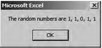
Create a VBA subroutine [call it Exercise3( ) ] which generates five random digits of either 1 or 0 and prints them out on the screen in a message box like the following: Microsoft Excel The random numbers are 1, 1, 0, 1, 1 OK
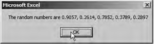
Create a VBA subroutine [call it Exercise2( ) ] which generates five random numbers and prints them out on the screen in a message box like the following: Use FormatNumber (Expression, NumDigitsAfterDecimal) to print out only four digits. Microsoft Excel The random numbers are 0.9057, 0.2614,
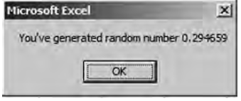
Create a VBA subroutine [call it Exercise1( ) ] which generates a random number and prints it on the screen in a message box that looks like this: Use the VBA keyword Rnd. Microsoft Excel You've generated random number 0.294659 OK
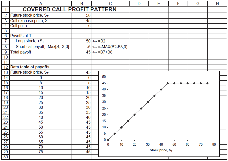
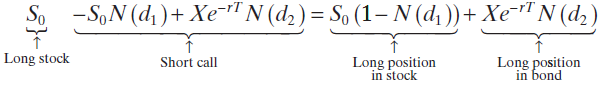
A covered call is a long stock and short call. The pattern of payoffs is given below: In this problem, you are asked to simulate the payoffs of a covered call over 52 weeks, with weekly updating of the positions. Start by deriving the formula for the covered call: Add together the Black-Scholes
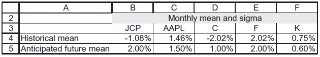
Using the data from the previous example, simulate 36 months of stock returns assuming the same variance-covariance structure as the historical returns. Notice that it doesn?t make sense to assume that the forward-looking expected monthly returns are the same as the historical returns. Instead, use
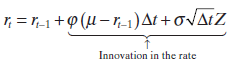
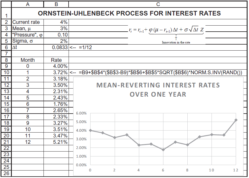
The previous example assumes that the risk-free rate is constant. An alternative, perhaps more plausible, model might be to assume that the risk-free rate is mean reverting, with a long-run mean. Under this assumption, if the current rate is above the long-run mean, the next period rate will tend
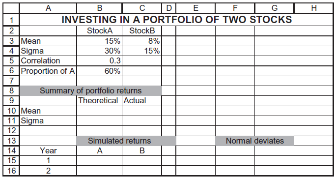
Consider a portfolio of two stocks whose statistical parameters are given below. Stock A: Annual mean return = 15%, annual standard deviation of return = 30%. Stock B: μ = 8%, σ= 15%. Correlation(A,B) = ρ = 0.3 An investor with a buy-and-hold strategy buys a portfolio composed of
Run a few of the lognormal price path simulations. Examine the price pattern for trends. Find one or more of the following technical patterns:support arearesistance areauptrend/downtrendhead and shoulders inverted head and shouldersdouble top/bottomrounded top/bottomtriangle (ascending,
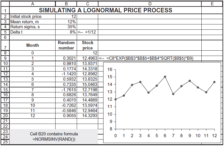
Use Norm.S.Inv(Rand( )) to produce a simulation of monthly stock prices, as illustrated below. 1 SIMULATING A LOGNORMAL PRICE PROCESS 2 Initial stock price 3 Mean return, m 4 Return sigma, s 5 Delta t 12 12% 35% 8%
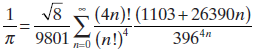
The great Indian mathematical genius Ramanujan showed that The n ! indicates the factorial: n! = n*(n - 1) = (n - 2) *...* 2 * 1 0! = 1 Excel?s function Fact computes the factorial. Use this series to construct a VBA function to value ?, where n is the number of terms in the series. Show that two
The first method for computing ? is: Use this formula to approximate ?. 1 =1+, 22 32 1 s+.. 6
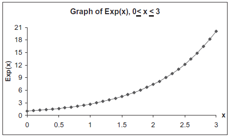
Use Monte Carlo to calculate the integral of the function Exp(x) for 0 Graph of Exp(x), 0
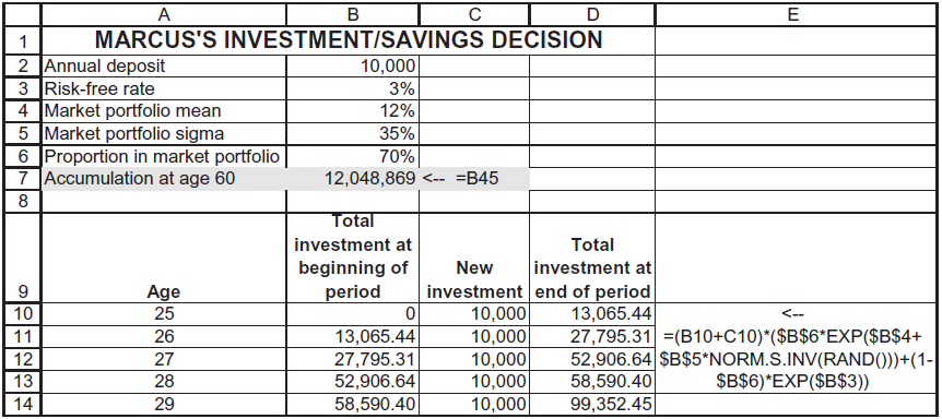
Marcus is 25 years old. He has a new job and intends to save $10,000 today and in each of the next 34 years (35 deposits altogether). He has decided on an investment policy in which he invests 30% of his assets in a risk-free bond with 3% continuously compounded annual interest and the remainder in
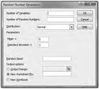
Stock price simulation: A stock?s price is lognormally distributed with mean ? = 15%. The current stock price is S0 = 35. Following the template on the spreadsheet, create 60 static standard normal deviates using Data|Data Analysis|Random Number Generation . Use these random numbers to simulate the
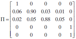
Consider the case of five possible rating states, A, B, C, D, and E. A, B, and C are initial bond ratings, D symbolizes first-time default, and E indicates default in the previous period. Assume that the transition matrix ? is: A 10-year bond issued today at par with an A rating is assumed to
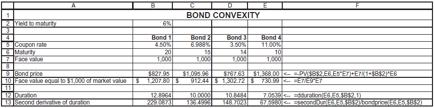
Set up a spreadsheet that enables you to duplicate the calculations of section 21.5 of this chapter. A. B E 1 BOND CONVEXITY 2 Yield to maturity 6% 3 Bond 2 6.988% Bond 3 3.50% Bond 4 11.00% 4 Bond 1 5 Coupon rate 6 Maturity 7 |Face value 4.50% 20 15 14 10 1,000 1,000 1,000 1,000 $1,368.00
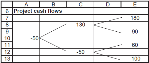
Consider the cash flows below: a. If the cost of capital is 30% and the risk-free rate is 5%, find the state prices which match the project?s NPV. b. If there exists an abandonment option so that we can change all negative cash flows to zero, value the project. A В E 6 Project cash flows 7 180
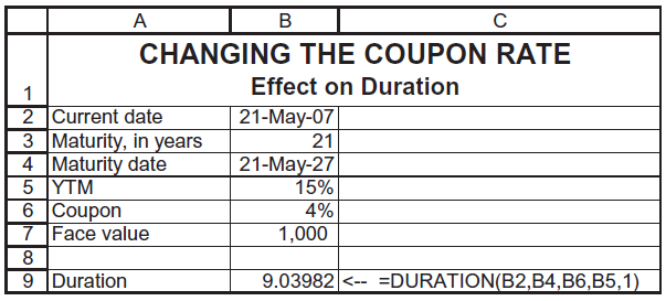
In the spreadsheet below, create a Data Table in which the duration is computed as a function of the coupon rate (coupon = 0%, 1%, ? , 11%). Comment on the relation between the coupon rate and the duration. A CHANGING THE COUPON RATE Effect on Duration 1 2 Current date 3 Maturity, in years 4
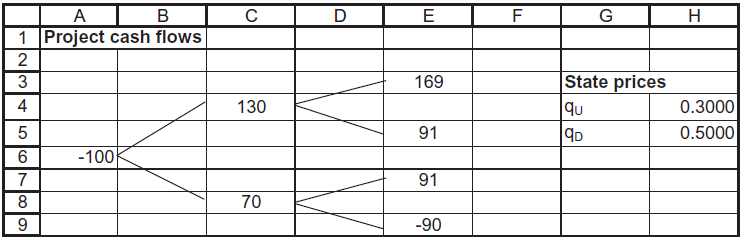
Consider the project whose cash flows are given below: a. Using the state prices, value the project. b. Suppose that at date 2 the project can be abandoned at no cost. What does this do to its value? c. Suppose that at any time the project can be sold for 100. Show the tree of cash flows and
Your company is considering purchasing 10 machines, each of which has the following expected cash flows (the entry in B3 of ? $550 is the cost of the machine): You estimate the appropriate discount rate for the machines as 25%. a. Would you recommend buying just one machine, if there are no
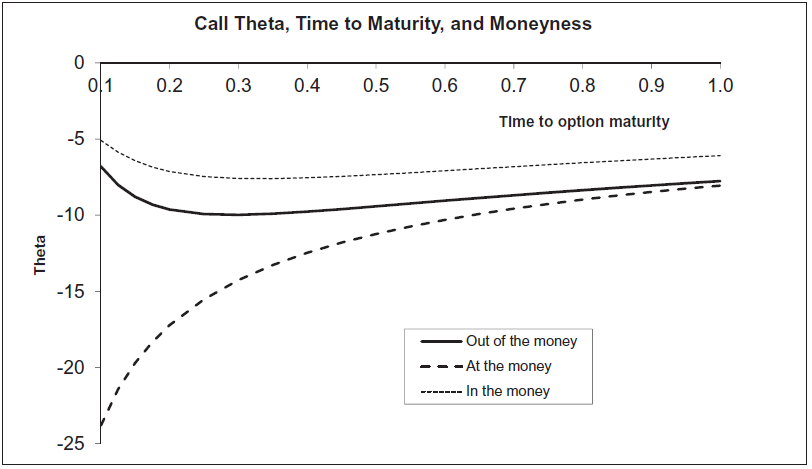
Figure 18.4 shows the call theta as a function of time to maturity. Produce a similar graph for puts. Call Theta, Time to Maturity, and Moneyness 01 0.2 0.3 0.4 0.5 0.6 0.7 0.8 0.9 1.0 Time to optlon maturlty -5 -10 -15 - Out of the money ---At the money ---- In the money -20 ---- -25 Theta
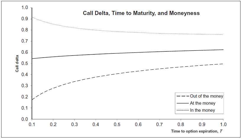
Produce a graph similar to the second panel of Figure 18.2 for puts. 1.0 Call Delta, Time to Maturity, and Moneyness 0.9 0.8 0.7 0.6 0.5 0.4 0.3 0.2 - Out of the money At the money 0.1 - In the money 0.0 0.1 0.2 0.3 0.4 0.5 0.6 0.7 0.8 0.9 1.0 Time to option expiration, T Call delta
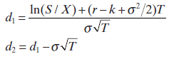
Note that you can also calculate the Black-Scholes put option premium as a percentage of the exercise price in terms of S/X: where Implement this in a spreadsheet. Find the ratio of S/X for which C/X and P/X cross when T = 0.5, ? = 25%, r = 10%. (You can use a graph or you can use Excel?s
Note that you can use the Black-Scholes formula to calculate the call option premium as a percentage of the exercise price in terms of S/X: where Implement this in a spreadsheet. C=SN(d))-Xe"T N(d»)→는=을N( C S -N(d)-eN(d2) X X
As shown in this chapter, Merton (1973) shows that for the case of an asset with price S paying a continuously compounded dividend yield k , this leads to the following call option pricing formula:C = Se?kTN(d1) ? Xe?rTN(d2),where a. Modify the BSCall and BSPut functions defined in this chapter
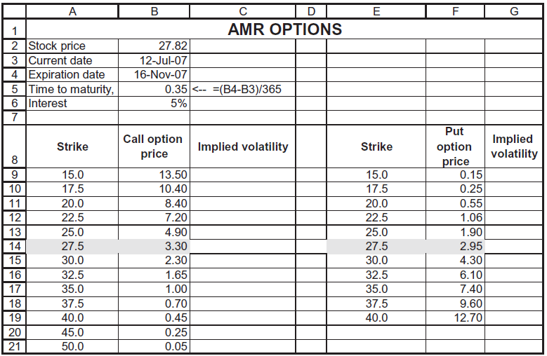
The table below gives prices for American Airlines (AMR) options on 12 July 2007. The option with exercise price X = $27.50 is assumed to be the at-the-money option. a. Compute the implied volatility of each option (use the functions CallVolatility and PutVolatility defined in the chapter). b.
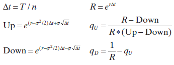
Here?s an advanced version of exercise 10. Consider an alternative parameterization of the binomial: Construct binomial European call and put option pricing functions in VBA for this parameterization and show that they also converge to the Black-Scholes formula.? At = T/n R= e" R- Down qu R* (Up-
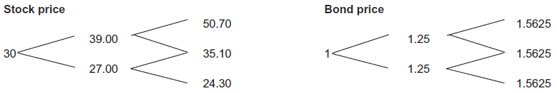
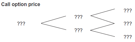
Consider the following three-date binomial model: ? In each period the stock price either goes up by 30% or decreases by 10%. ? The one-period interest rate is 25% a. Consider a European call with X = 30 and T = 2. Fill in the blanks in the tree: b. Price a European put with X = 30 and T =
Consider the following 2-period binomial model, in which the annual interest rate is 9% and in which the stock price goes up by 15% per period or down by 10%: a. Price a European call on the stock with exercise price 60. b. Price a European put on the stock with exercise price 60. c. Price an
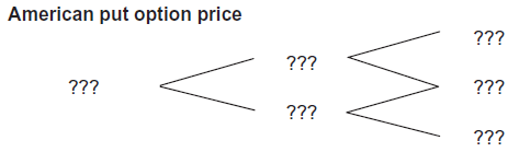
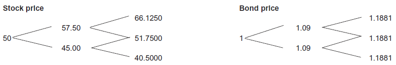
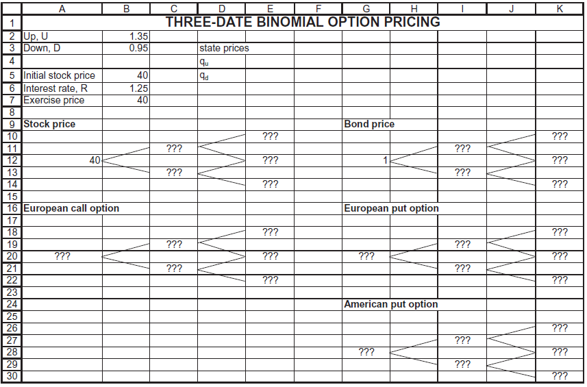
Fill in all the cells labeled ??? in the following spreadsheet: Why is there no additional pricing tree for an American call option? D E THREE-DATE BINOMIAL OPTION PRICING 1.35 A K 1 2 Up, U 3 Down, D state prices qu 0.95 4 5 Initial stock price 6 Interest rate, R 7 Exercise price 40 1.25 40 9
In exercise 1, compute the state prices qU and qD, and use these prices to calculate the value today of a one-year put option on the stock with exercise price $30. Show that put-call parity holds: That is, using your answer from this problem and the previous problem, show that: X = Stock price
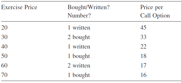
Consider the following option strategy, which consists only of calls: a. Draw the profit diagram for this strategy. b. The prices given include one violation of an arbitrage condition. Identify this violation and explain. Exercise Price Bought/Written? Price per Number? Call Option 20 1 written
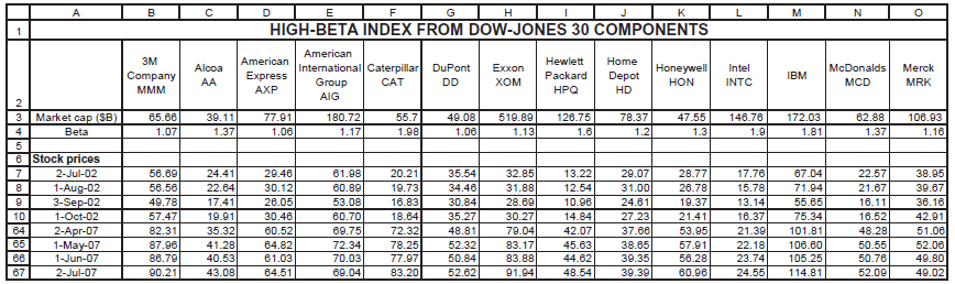
You have decided to create your own index of higher-beta components of the Dow-Jones 30 Industrials. Using Yahoo ? s stock screener, you come up with the data below. a. Compute the variance-covariance matrix of returns. b. Assuming that the risk-free rate is 5.25% annually (= 5.25%/12 = 0.44%
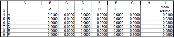
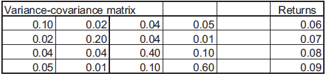
Given the data below: a. Calculate the efficient frontier assuming no short sales are allowed. b. Calculate the efficient frontier assuming that short sales are allowed. c. Graph both frontiers on the same set of axes. A В Mean А B D E F returns 4 JA 5 B 6 JC 7 D 8 JE 0.0100 0.0000 0.0000 0.0000
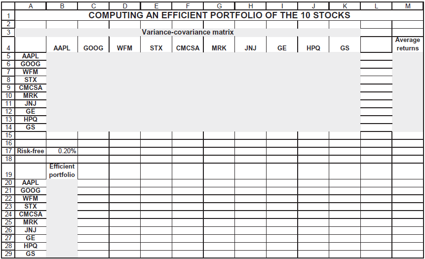
Compute the variance-covariance matrix for the 10 stocks. Using the monthly average returns and a monthly risk-free interest rate of 0.20%, compute an efficient portfolio. Here?s the template: DIE F COMPUTING AN EFFICIENT PORTFOLIO OF THE 10 STOCKS A В G H M 1 Variance-covariance matrix Average
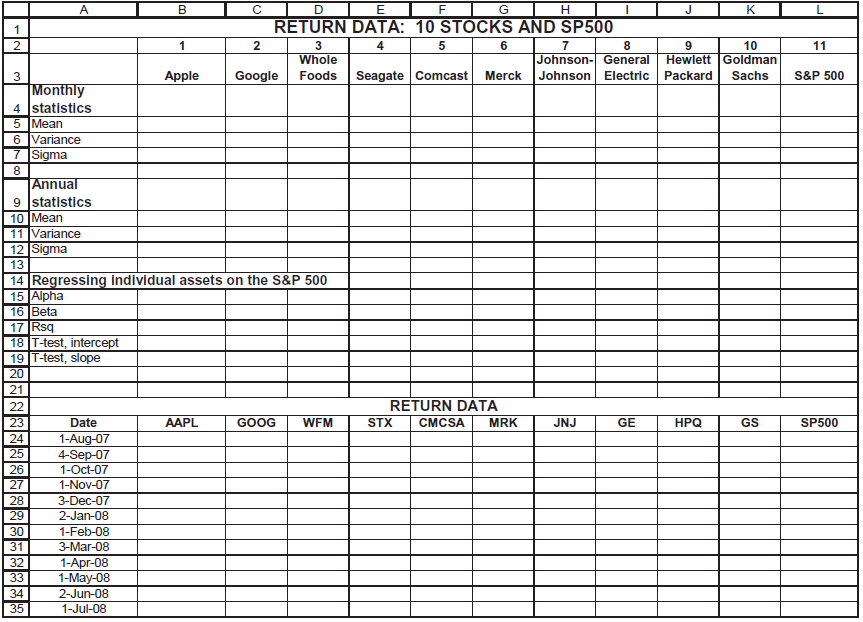
Fill in the template file below. A B F G K RETURN DATA: 10 STOCKS AND SP500 1 1 2 3 4 6 7 8. 10 11 Whole Hewlett Goldman Johnson- General Johnson Electric 3 Apple Google Foods Seagate Comcast Merck Packard Sachs S&P 500 |Monthly 4 statistics 5 Mean 6 Variance 7 Sigma 8. Annual 9 statistics 10 Mean
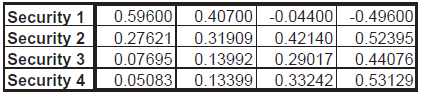
In a well-known paper, Roll (1978) discusses tests of the SML in a four-asset context: a. Derive two efficient portfolios in this 4-asset model and draw a graph of the efficient frontier. b. Show that the following four portfolios are efficient by proving that each is a convex combination of the
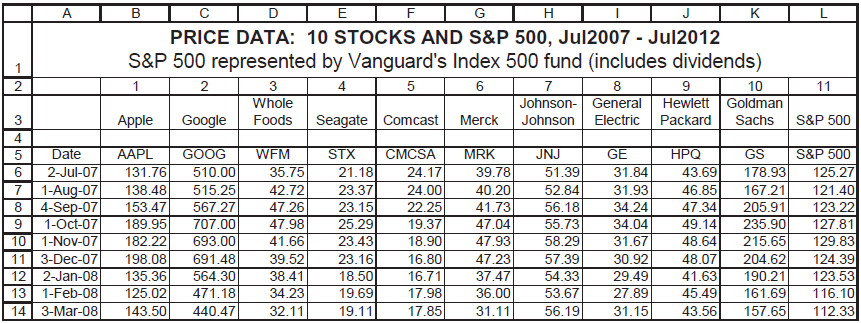
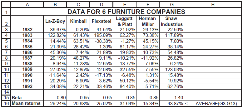
Below you will find annual return data for six furniture companies for the years 1982? 1992. Use these data to calculate the variance-covariance matrix of the returns. The remaining exercises refer to the data in the tab Price data on the exercise spreadsheet that accompanies this book. This tab
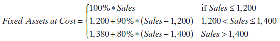
Back to the basic model of section 5.1. Suppose that the fixed assets at cost follow the following step function: Incorporate this function into the model. if Sales
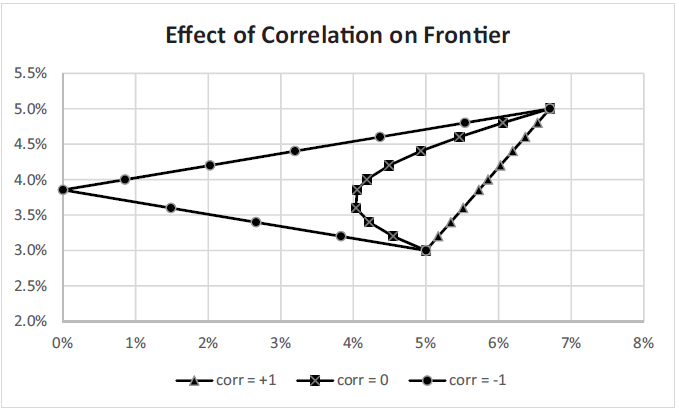
Assets A and B have the means and variances indicated in the exercise file. Graph three cases, ρAB = −1, 0, + 1 on one set of axes, producing the following chart: Effect of Correlation on Frontier 5.5% 5.0% 4.5% 4.0% 3.5% 3.0% 2.5% 2.0% 0% 1% 2% 3% 4% 5% 6% 7% 8% - corr = +1 corr = 0 corr = -1
Stock price simulation: A stock’s price is lognormally distributed with mean μ = 15% and σ = 50%. The current stock price is S0 = 35. Following the template on the spreadsheet, create 60 dynamic standard normal deviates using Norm.S.Inv(Rand( )). Use these random numbers to simulate the stock
Compute the returns of the data and the statistics for each of the assets (mean return, variance and standard deviation of return, beta).
The model of section 5.1 includes costs of goods sold but not selling, general, and administrative (SG&A) expenses. Suppose that the firm has $200 of these expenses each year, irrespective of the level of sales.a. Change the model to accommodate this new assumption. Show the resulting profit
On 12 July 2007 call and put options to purchase and sell 10,000 euros at $1.37 per euro are traded on the Philadelphia options exchange. The options’ expiration date is 20 December 2007. If the dollar interest rate is 5%, the euro interest rate is 4.5% and the volatility of the euro is 6%, what
Tareq and Jamillah are playing with a single die for money. According to the rules of their game, Tareq pays Jamillah $0.50 at the start of every round, before they throw a die. They then throw the die; if it falls on an even number, Jamillah pays that amount in dollars to Tareq, and if it falls on
Marcus decides that he needs at least $2 million by the time he hits 60.• Run 100 simulations in order to determine the approximate probability of achieving this goal.• Compute the average and standard deviation of the terminal wealth.• Create a Data Table to determine the relation between
Martha is playing a coin-toss game in which she tosses two coins. The probability of heads on the second coin is correlated with correlation ρ = 0.6 with the probability of heads on the first coin. In this particular game, Martha wins $1 for each heads that she tosses.• Model one round of 2 coin
In section 25.2 we designed a macro which calculates the value of π using Monte Carlo and which updates the screen every iteration. Modify the macro so that it updates the screen only every 1,000 iterations.• Use the VBA function Mod . From the VBA help menu, note that this function has syntax a
In the previous exercise, put a “switch” on the spreadsheet itself, which controls the updating of the macro (whether to update, yes or no, and how often to update).
One of the messages of this chapter is that while Monte Carlo is a clever method of calculation, it shouldn’t be used when some better method exists. The MC valuation of π in section 25.2, for example, converges very slowly. It’s a crummy way to compute π, since there are well-known methods
Expand the previous exercise and use Norm.S.Inv(Rand( )) to produce a simulation of daily stock prices for 250 days (approximately 1 year of trading days).
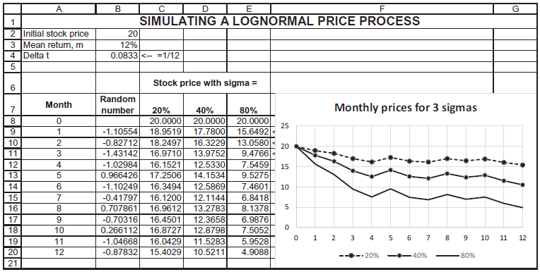
Re-create the spreadsheet below. Play with the spreadsheet (each press of F9 will recompute the numbers) to convince yourself that higher σ means a more volatile price path for the stock.
Write a VBA program which reproduces the lognormal frequency distribution for an arbitrary number of runs. That is, this program should• Produce N normal random deviates.• For each deviate produce a lognormal price relative exp [μΔt + σZ√Δt].• Classify each price relative into a set of
The exercise file for this chapter contains daily price data for the S&P 500 index and for Abbott Laboratories for the 3 months April–June 2007. Use these data to compute the annual average, variance, and standard deviation of the logarithmic returns for the S&P and for Abbott. What is
The exercise file for this chapter gives daily returns from 1987–2012 for the Vanguard Index 500 fund (VFINX). This is a fund that tracks the S&P 500, but the returns include dividends (as opposed to ∧ GSPC, the index tracker).• Compute the overall daily return statistics: average and
Reconsider the problem above. Assume that the risk-free rate is 4% and that the investor (still buy-and-hold) invests in a portfolio composed of 50% risk-free and 50% invested in the 60/40 portfolio of A and B. Compare the theoretical to the simulated returns.
The disk that accompanies this book gives 5 years of monthly price data for five U.S. stocks.• Compute the monthly returns for the stocks.• Compute the stocks’ average monthly returns and standard deviations.• Compute the variance-covariance matrix for the stock returns.• Compute the
You are a portfolio manager, and you want to invest in an asset having σ = 40%. You want to create a put on the investment so that at the end of the year you have losses no greater than 5%. Since there is no put on this specific asset, you plan to create a synthetic put by engaging in a dynamic
Simulate the above strategy, assuming weekly rebalancing of the portfolio.
Go back to the numerical example of section 29.5. Write a VBA function which solves for the implied asset value Va. Then use this function to create a graph showing the trade-off between the implied asset value and the asset volatility.
You have been offered the chance to purchase stock in a firm. The seller wants $55 per share, but offers to repurchase the stock at the end of one half year for $50 per share. If the σ of the share’s log returns is 80% determine the true value per share. Assume that the interest rate is 10%.
Section 29.2 discusses the cashless replication of a call. Use the same logic to program in a spreadsheet the replication of a put.
Using Data Table graph the function sin(x * y) for x = 0, 0.2, 0.4, … 1.8, 2 and y = 0, 0.2, 0.4, … 1.8, 2. Use the “Surface” graph option to make a three-dimensional graph of the function.
Boris and Tareq are tossing coins. For each toss, if the coin falls on heads, Tareq wins $1. If the coin falls on tails, Tareq pays Boris $1.• Simulate 10 rounds of this game, showing Tareq’s cumulative winnings.• Use Data Table on a blank cell to simulate 25 games of 10 rounds each, showing
Maria and Shavit are tossing coins. Their game works as follows:On the first toss, if the coin falls on heads, Shavit pays Maria $1 (and vice versa).On each successive toss:If the coin falls on heads and Maria is ahead, Shavit pays her the square of her previous winnings.If the coin falls on heads
Use a homemade array function to multiply the vector {1,2,3,4,5} times the constant 3.
For the problem above: Use an array function to create a matrix with zeros on the diagonal and the covariances off-diagonal.
The exercise Excel notebook gives data for three mutual funds. Compute the discrete annual returns for each fund and then use an array function to compute the compound annual return over the period. Recall that discretely compounded, the return in year t is (Fund value t / Fund valuet−1) − 1.
A bank offers different interest rates on loans. The rate is based on the size of the periodical repayment ( CF i ) and the following table. Write a present value function BankPV(CF, r) so that it reflects the present value of a loan in the bank. The function should be useable as a worksheet
A bank offers different interest rates on deposit accounts. The rate is based on the size of the periodical deposit ( CF i ) and the following table. Write a future value function BankFV(CF, r). The function should be useable as a worksheet function. CF could be either a row range or a column
Another bank offers 1% increase in interest rate to savings accounts with a balance of more than 10,000.00. Write a future value function Bank1FV(CF, r) that reflects this policy. The function should be useable as a worksheet function. CF could be either a row range or a column range.
Rewrite the subroutine in the previous exercise so it deals properly with the Cancel button.• A simple version of the new subroutine will abort the subroutine if Cancel is clicked in any stage.• A more sophisticated version of the new subroutine will allow the user to reenter the data from
Write a subroutine that multiplies all cells in the current region by 2.
Rewrite the subroutine in exercise 3 so that its action is dependent on the cell’s contents.• If the cell contents is a formula, it will be replaced by the same formula multiplied by 2.• If the cell contents is a number, it will be replaced by a number equal to the old number multiplied by
Rewrite the subroutine in exercise 4 so that it uses another method (the correct one) to detect the existence of a formula in a cell. Look at the different properties of the Range object in the Help file.
The Selection object represents the current selection in the worksheet. Selection is usually, and for our purposes always, a Range object. Rewrite the subroutine in exercise 6 so that it works on a selected range.Note the following:If the selected range is a single cell, activate the subroutine in
Many states have daily lotteries, which are played as follows: Sometime during the day, you buy a lottery ticket, on which the seller inscribes a number you choose, between 000 and 999. That night there is a drawing on television in which a three-digit number is drawn. If the number on your ticket
Define AmodB as the remainder when A is divided by B. For example 36mod25 = 11. Excel has this function; it is written Mod(A,B) . Now here is another random-number generator:• Let X0 = seed .• Let Xn + 1 = (7*Xn)mod108.• Let Un + 1 = Xn+1/108.The list of numbers U1 , U2, … are the
Write a VBA Exercise1(seed) that produces a random number based on a Seed and the rule of the previous exercise.
Here is a random-number generator you can make yourself:• Start with some number, Seed.• Let X1 = Seed + π. Let X2 = e5+In(X1).• The first random number is Random = X2 − Integer (X2), where Integer (X2) is the integer part of X2.• Repeat the process, letting Seed = Random .Run 1,000 of
An underwriter issues a new 7-year C-rated bond at par. The anticipated recovery rate in default of the bond is expected to be 55%. What should be the coupon rate on the bond so that its expected return is 9%? Assume the transition matrix of exercise 2.
An underwriter issues a new 7-year B-rated bond with a coupon rate 9%. If the expected rate of return on the bond is 8%, what is the bond ’ s implied recovery percentage λ ? Assume the transition matrix given in section 23.5.
Using the transition matrix of the previous problem: A C-rated bond is selling at par on 18 July 2007. The bond ’ s maturity is 17 July 2017, it has a coupon (paid annually on 17 July) of 11%, and it has a recovery percentage of λ = 67%. What is the bond’s expected return?
A newly issued bond with 1 year to maturity has a price of 100, which equals its face value. The coupon rate on the bond is 15%; the probability of default in 1 year is 35%; and the bond’s payoff in default will be 65% of its face value.a. Calculate the bond’s expected return.b. Create a data
Prove that the duration of a portfolio is the weighted average duration of the portfolio assets.
Rewrite the formula DDuration in section 20.5, so that if the timeToFirstPayment α is not inserted, then α automatically defaults to 1.
On 23 January 1987, the market price of a West Jefferson Development Bond was $1,122.32. The bond pays $59 in interest on 1 March and 1 September of each of the years 1987–1993. On 1 September 1993, the bond is redeemed at its face value of $1,000. Calculate the yield to maturity of the bond and
Replicate the two graphs in section 20.5.
A pure discount bond with maturity N is a bond with no payments at times t = 1, … , N − 1; at time t = N , a pure discount bond has a single terminal payment of both principal and interest. What is the duration of such a bond?
“Duration can be viewed as a proxy for the riskiness of a bond. All other things being equal, the riskier of two bonds should have lower duration.” Check this claim with an example. What is its economic logic?
What is the effect on a bond’s duration of increasing the bond’s maturity? As in the previous example, use a numerical example and plot the answer. Note that as N → ∞, the bond becomes a consol (a bond that has no repayment of principal but an infinite stream of coupon payments). The
Suppose that the market portfolio has mean μ = 15% and standard deviation σ = 20%.a. If the risk-free rate of interest is 8% calculate the 1-period state prices for an “up” and a “down” state.b. Show the effect (in a data table) of the risk-free rate on the state prices.c. Show the effect
Your company is considering the purchase of a new piece of equipment. The equipment costs $50,000 and your analysis indicates that the PV of the future cash flows from the equipment is $45,000. Thus the NPV of the equipment is − $5,000. This estimated NPV is based on some initial numbers provided
Although θ is generally negative, there are cases (typically of high interest rates) where it can be positive:• An in-the-money put with a high interest rate• An in-the-money call on a currency which has a high interest rate (or—equivalently—an in-the-money call on a stock with a very high
Consider a structured security of the following type: The purchaser invests $1,000 and in three years gets back the initial investment plus 95% of the increase in a market index whose current price is 100. The interest rate is 6% per year, continuously compounded. Assuming the security is fairly
Use the Excel Solver to find the stock price for which there is the maximum difference between the Black-Scholes call option price and the option’s intrinsic value. Use the following values: S = 45, X = 45, T = 1, σ = 40%, r = 8%.
Re-examine the X = 17.50 call for AMR in the previous exercise.a. Is the call correctly priced?b. What price would be necessary for this call in order for the implied volatility to be 60%?
Produce a graph comparing a put’s intrinsic value [ = max( X − S ,0)] and its Black-Scholes price. From this graph you should be able to deduce that it may be optimal to exercise early a put priced by the Black-Scholes formula.
Produce a graph comparing a call’s intrinsic value [defined as max(S − X , 0)] and its Black-Scholes price. From this graph you should be able to deduce that it is never optimal to exercise early a call priced by the Black-Scholes.
Use the data from exercise 1 and Data|Table to produce graphs that show:• The sensitivity of the Black-Scholes call price to changes in the initial stock price S.• The sensitivity of the Black-Scholes put price to changes in σ.• The sensitivity of the Black-Scholes call price to changes in

Showing 700 - 800 of 888

1
2
3
4
5
6
7
8
9

Step by Step Answers

Services

Sitemap
Fun
Definitions
Become Tutor
Used Textbooks
Study Help Categories
Recent Questions
Expert Questions
Campus Wear
Sell Your Books

Company Info

Security
Copyrights
Privacy Policy
Terms & Conditions
SolutionInn Fee
Scholarship
Online Quiz
Give Feedback, Get Rewards

Get In Touch

About Us
Contact Us
Career
Jobs
FAQ
Student Discount
Campus Ambassador

Secure Payment

Download Our App

© 2026 SolutionInn. All Rights Reserved