New Semester Started Get 50% OFF Study Help! --h --m --s Claim Now

Question Answers

Textbooks

Find textbooks, questions and answers

Oops, something went wrong!

Change your search query and then try again

Result Not Found

Books FREE
Study Help
Tutors
AI Study Planner NEW
Sell Books

Search
Sign In
Register

study help
business
practical management science

Practical Management Science 5th Edition Wayne L. Winston, Christian Albright - Solutions

Two construction companies are bidding against one another for the right to construct a new community center building in Bloomington, Indiana. The first construction company, Fine Line Homes, believes that its competitor, Buffalo Valley Construction, will place a bid for this project according to
A buyer for a large department store chain must place orders with an athletic shoe manufacturer six months prior to the time the shoes will be sold in the department stores. The buyer must decide on November 1 how many pairs of the manufacturer’s newest model of tennis shoes to order for sale
An investor with $10,000 available to invest has the following options: (1) he can invest in a risk-free savings account with a guaranteed 3% annual rate of return; (2) he can invest in a fairly safe stock, where the possible annual rates of return are 6%, 8%, or 10%; or (3) he can invest in a more
Techware Incorporated is considering the introduction of two new software products to the market. The company has four options regarding these products: introduce neither product, introduce product 1 only, introduce product 2 only, or introduce both products.Research and development costs for
Starting with the finished version of Example 9.3, change the fixed marketing cost to $4000 (really $4 million) in cell B5, and change the decision criterion to “maximize expected utility,” using an exponential utility function with risk tolerance $5000 (really $5 million). Display certainty
Starting with the finished version of Example 9.2, change the decision criterion to “maximize expected utility,” using an exponential utility function with risk tolerance $5000 (really $5 million). Display certainty equivalents on the tree.a. Keep doubling the risk tolerance until the
Starting with the finished version of Example 9.2, change the decision criterion to “maximize expected utility,” using an exponential utility function with risk tolerance $5000 (really $5 million). Display certainty equivalents on the tree.
You saw in Example 9.4 how Acme prefers to abandon the product when the risk tolerance in cell B12 is $5000 (really $5 million). This is despite the fact that the EMV from continuing with the product is well above 0. Using this same risk tolerance, experiment with the sales volume from a great
Using the finished version of the file for Example 9.4, use a data table to perform a sensitivity analysis on the risk tolerance. Specifically, let the risk tolerance in cell B12 vary from $10,000 to $100,000 and keep track of two outputs in the data table, the TRUE/ FALSE value in cell B14 and the
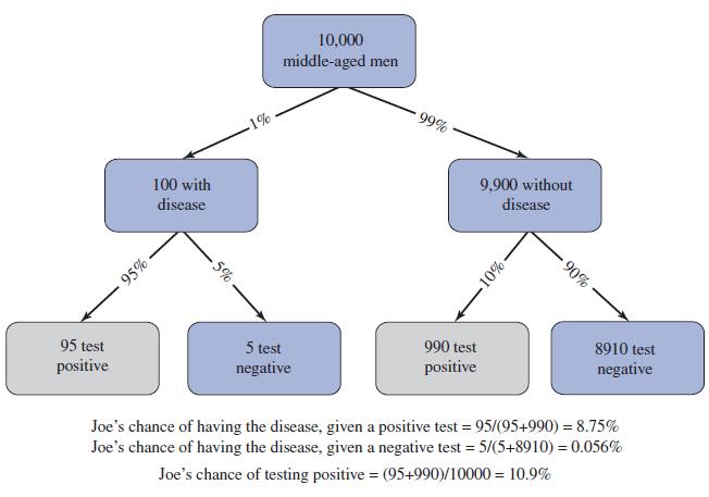
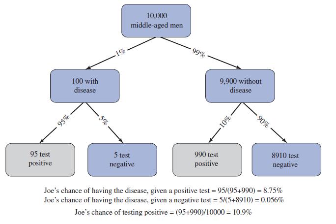
The terms prior and posterior are relative. Assume that the test in Figure 9.17 (and in the file Bayes Rule for Disease.xlsx) has been performed, and the outcome is positive, which leads to the posterior probabilities shown. Now assume there is a second test, independent of the first, that can be
The terms prior and posterior are relative. Assume that the test in Figure 9.17 (and in the file Bayes Rule for Disease.xlsx) has been performed, and the outcome is positive, which leads to the posterior probabilities shown. Now assume there is a second test, independent of the first, that can be
The model in Example 9.3 has only two market outcomes, good and bad, and two corresponding predictions, good and bad. Modify the decision tree by allowing three outcomes and three predictions, good, fair, and bad. You can change the inputs to the model (monetary values and probabilities) in any
In Example 9.2, a technological failure implies that the game is over—the product must be abandoned. Change the problem so that there are two levels of technological failure, each with probability 0.1. In the first level, Acme can pay a further development cost D to fix the product and make it a
If you examine the decision tree in Figure 9.12 (or any other decision trees from PrecisionTree), you will see two numbers (in blue font) to the right of each end node. The bottom number is the combined monetary value from following the corresponding path through the tree. The top number is the
Starting with the finished version of the file for Example 9.3, change the fixed cost in cell B5 to $4000. Then get back into PrecisionTree’s One-Way Sensitivity Analysis dialog box and add three more inputs. (These will be in addition to the two inputs already there, cells B9 and B5.) The first
The finished version of the file for Example 9.3 contains two “Strategy B9” sheets. Explain what each of them indicates and how they differ.
In using Bayes’ rule for the presence of a disease (see Figure 9.17 and the file Bayes Rule for Disease.xlsx), we assumed that there are only two test results, positive or negative. Suppose there is another possible test result, “maybe.” The 2 x 2 range B9:C10 in the file should now be
In Example 9.2, use a two-way PrecisionTree sensitivity analysis to examine the changes in both of the two previous problems simultaneously. Let the probability of technological success vary from 0.6 to 0.9 in increments of 0.05, and let the fixed cost of development vary as indicated in the
In Example 9.2, the fixed costs are split $4 million for development and $2 million for marketing. Perform a sensitivity analysis where the sum of these two fixed costs remains at $6 million but the split changes. Specifically, let the fixed cost of development vary from $1 million to $5 million in
In Example 9.2, Acme’s probability of technological success, 0.8, is evidently large enough to make “continue development” the best decision. How low would this probability have to be to make the opposite decision best?
Use PrecisionTree to solve problem 7 of the previous section.Problem 7Sometimes a "single-stage" decision can be broken down into a sequence of decisions, with no uncertainty resolved between these decisions. Similarly, uncertainty can sometimes be broken down into a sequence of uncertain outcomes.
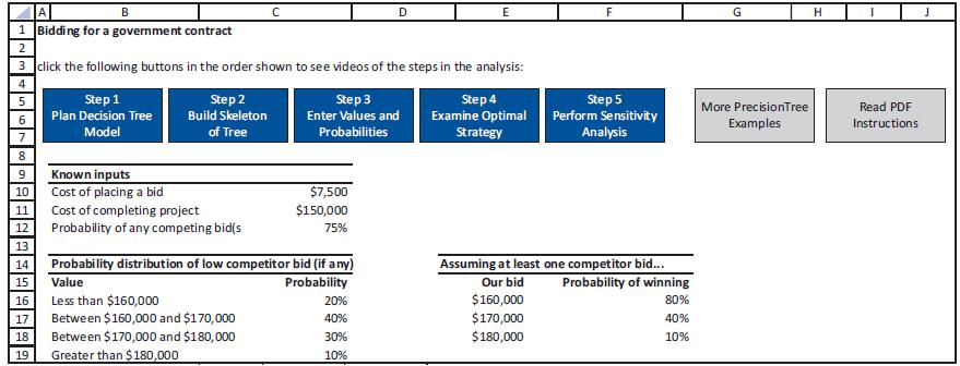
Use PrecisionTree’s Sensitivity Analysis tools to perform the sensitivity analysis requested in problem 5 of the previous section. (Watch the Step 5 video in Figure 9.10 if necessary.)Figure 9.10 A B E G. H 1 Bidding for a government contract 2 3 click the following buttons in the order shown to
For the decision problem in Figure 9.1, use data tables to perform the following sensitivity analyses. The goal in each is to see whether decision 1 continues to have the largest EMV. In each part, provide a brief explanation of the results.a. Let the payoff from the best outcome, the value in cell
The 30 teams in the NBA are each assigned to one of six divisions, where each division has five teams. Suppose the goal is to assign the teams to divisions so that the average distance among teams in the divisions is minimized. In other words, the goal is to make the assignments so that teams
Based on Schrage (1997). The file P08_05.xlsx lists the size of the four main markets for Excel, Word, and the bundle of Excel and Word. (We assume that Microsoft is willing to sell Excel or Word separately, and it is willing to sell a package with Excel and Word only.) It also shows how much
Modify the function in Example 8.1 so that it becomes f (x) = x sin(x) for 0 ≤ x ≤ 30. (Here, sin(x) is the sine function from trigonometry. You can evaluate it with Excel’s SIN function.) Plot a lot of points from 0 to 30 to see what the graph of this function looks like. Then use GRG
Consider the sports ratings model in section 7.6. If you were going to use the approach used there to forecast future sports contests, what problems might you encounter early in the season? How might you resolve these problems?
Consider the sports ratings model in section 7.6. If you were going to give more recent games more weight, how might you determine whether the weight given to a game from k weeks ago should be, say, (0.95)k or (0.9)k?
You are given that the two nonhypotenuse sides of a right triangle add up to 10 inches. What is the maximum area of the triangle? Can you generalize this result?
Based on Grossman and Hart (1983). A salesperson for Fuller Brush has three options: (1) quit, (2) put forth a low level of effort, or (3) put forth a high level of effort. Suppose for simplicity that each salesperson will sell $0, $5000, or $50,000 worth of brushes. The probability of each sales
Continuing the previous problem, find the portfolio that achieves an expected monthly return of at least 1% and minimizes portfolio variance. Then use SolverTable to sweep out the efficient frontier, as in Example 7.9. Create a chart of this efficient frontier from your SolverTable results. What
This problem continues using the data from the previous problem. The file P07_40.xlsx includes all of the previous data and contains investment weights in row 3 for creating a portfolio. These fractions are currently all equal to 1/27, but they can be changed to any values you like, as long as they
The file P07_39.xlsx contains historical monthly returns for 27 companies. For each company, calculate the estimated mean return and the estimated variance of return. Then calculate the estimated correlations between the companies’ returns. Note that “return” here means monthly return. (Hint:
By the time you are reading this, the 2014 NFL season will have finished, and the results should be available at http://www.pro-football-reference.com/years/ 2014/games.htm. Do whatever it takes to get the data into Excel in the format of this example. Then, use Solver to find the ratings and
The file P07_31.xlsx contains scores on all of the regular- season games in the NBA for the 2012–2013 basketball season. Use the same procedure as in Example 7.8 to rate the teams. Then sort the teams based on the ratings. Do these ratings appear to be approximately correct? (You might recall
Carry out the suggestion in Modeling Issue 2. That is, use a weighted sum of squared prediction errors, where the weight on any game played k weeks ago is 0.95k. You can assume that the ratings are being made right after the final regular games of the season (in week 17), so for these final games,
Carry out the suggestion in Modeling Issue 3. That is, find the ratings of the 2013 NFL teams using the sum of absolute prediction errors as the criterion to minimize. Discuss any differences in ratings from this method and the method used in Example 7.8.
The file P07_28.xlsx lists the scores of all NFL games played during the 2008 season. Use this data set to rank the NFL teams from best to worst.
In the solution to the advertising selection model in Example 7.6, we indicated that the women 36 to 55 group is a bottleneck in the sense that the company needs to spend a lot more than it would otherwise have spent to meet the constraint for this group. Use SolverTable to see how much this
The file P06_92.xlsx lists the distances between 21 U.S. cities. You want to locate liver transplant centers in a subset of these 21 cities.a. Suppose you plan to build four liver transplant centers and your goal is to minimize the maximum distance a person in any of these cities has to travel to a
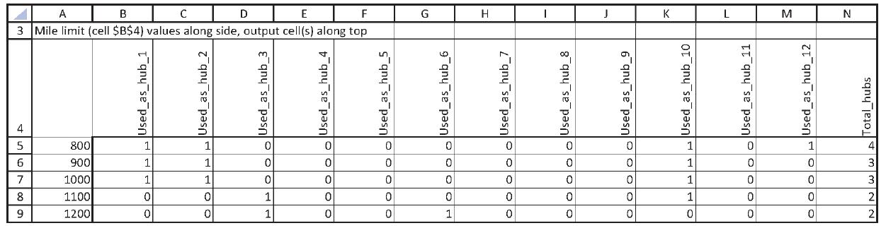
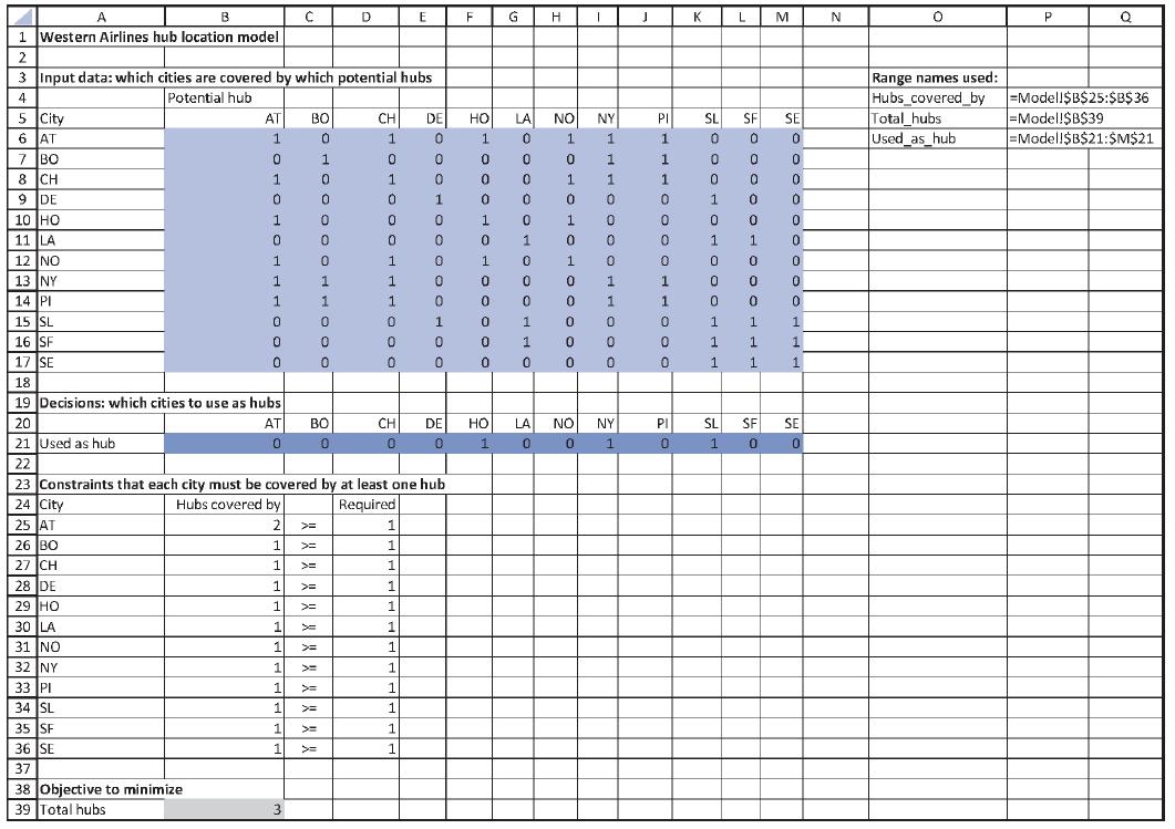
How hard is it to expand a set-covering model to accommodate new cities? Answer this by modifying the model in Figure 6.25. (See the file Locating Hubs with Distances.xlsx.) Add several cities that must be served: Memphis, Dallas, Tucson, Philadelphia, Cleveland, and Buffalo. You can look up the
Set-covering models such as the original Western model in Figure 6.22 often have multiple optimal solutions. See how many alternative optimal solutions you can find. Of course, each must use three hubs because this is optimal. Use various initial values in the decision variable cells and then run
In the original Western set-covering model in Figure 6.22, we assumed that each city must be covered by at least one hub. Suppose that for added flexibility in flight routing, Western requires that each city must be covered by at least two hubs. How do the model and optimal solution change?Figure
In the original Western set-covering model in Figure 6.22, we used the number of hubs as the objective to minimize. Suppose instead that there is a fixed cost of locating a hub in any city, where these fixed costs can possibly vary across cities. Make up some reasonable fixed costs, modify the
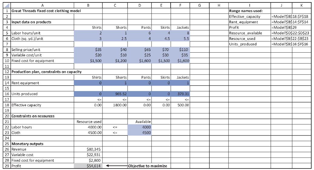
In the optimal solution to the Great Threads model, the labor hour and cloth constraints are both binding—the company is using all it has.a. Use SolverTable to see what happens to the optimal solution when the amount of available cloth increases from its current value. (You can choose the range
In the Great Threads model, we didn’t constrain the production quantities in row 16 to be integers, arguing that any fractional values could be safely rounded to integers. See whether this is true. Constrain these quantities to be integers and then run Solver. Are the optimal integer values the
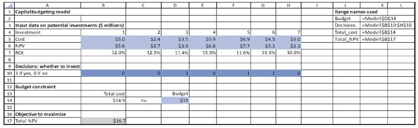
Expand and then solve the capital budgeting model in Figure 6.5 so that 20 investments are now possible. You can make up the data on cash requirements, NPVs, and the budget, but use the following guidelines:• The cash requirements and NPVs for the various investments can vary widely, but the ROIs
Solve the previous problem using the input data in the file P06_02.xlsx.Previous problemIn the capital budgeting model in Figure 14.40, we supplied the NPV for each investment. Suppose instead that you are given only the streams of cash inflows from each investment shown in the file
In the VanBuren machine replacement problem, the company’s current policy is to keep a machine at least four quarters but no more than 12 quarters. Suppose instead that the company imposes no upper limit on how long it will keep a machine; its only policy requirement is that a machine must be
In the VanBuren machine replacement problem, the company’s current policy is to keep a machine at least 4 quarters but no more than 12 quarters. Suppose this policy is instead to keep a machine at least 5 quarters but no more than 10 quarters. Modify the spreadsheet model appropriately. Is the
Based on Gaballa and Pearce (1979). Northwest Airlines has determined that it needs the number of ticket agents during each hour of the day listed in the file P04_75.xlsx. Workers work nine-hour shifts, one hour of which is for lunch. The lunch hour can be either the fourth or fifth hour of their
A large U.S. drug company, Pharmco, has 100 million yen coming due in one year. Currently the yen is worth $0.01. Because the value of the yen in U.S. dollars in one year is unknown, the value of this 100 million yen in U.S. dollars is highly uncertain. To hedge its risk, Pharmco is thinking of
You are playing Serena Williams in tennis, and you have a 42% chance of winning each point.a. Use simulation to estimate the probability you will win a particular game. Note that the first player to score at least four points and have at least two more points than his or her opponent wins the
The file P14_52.xlsx contains data on a motel chain’s revenue and advertising.a. Use these data and multiple regression to make predictions of the motel chain’s revenues during the next four quarters. Assume that advertising during each of the next four quarters is $50,000.b. Use simple
Confederate Express is attempting to determine how its monthly shipping costs depend on the number of units shipped during a month. The file P14_46.xlsx contains the number of units shipped and total shipping costs for the past 15 months.a. Use regression to determine a relationship between units
Let Yt be the sales during month t (in thousands of dollars) for a photography studio, and let Pt be the price charged for portraits during month t. The data are in the file P14_39.xlsx.a. Use regression to fit the following model to these data: Yt = a + b1 Pt + b2Yt–1. This says that current
A trucking firm must decide at the beginning of the year on the size of its trucking fleet. If on a given day the firm does not have enough trucks, the firm will have to rent trucks from a rental company. Discuss how you would determine the optimal size of the trucking fleet?
An exchange curve can be used to display the trade-offs between the average investment in inventory and the annual ordering cost. To illustrate the usefulness of a trade-off curve, suppose that a company must order two products with the attributes shown in the file P12_66.xlsx.a. Draw a curve that
A company inventories two items. The relevant data are shown in the file P12_65.xlsx. Determine the optimal inventory policy if no shortages are allowed and if the average investment in inventory is not allowed to exceed $700. If this constraint could be relaxed by $1, by how much would the
Based on Riccio et al. (1986). The borough of Staten Island has two sanitation districts. In district 1, street litter piles up at an average rate of 2000 tons per week, and in district 2, it piles up at an average rate of 1000 tons per week. Each district has 500 miles of streets. Staten Island
A firm knows that the price of the product it is ordering is going to increase permanently by X dollars. It wants to know how much of the product it should order before the price increase goes into effect. Here is one approach to this problem. Suppose the firm places one order for Q units before
A newspaper has 500,000 subscribers who pay $4 per month for the paper. It costs the company $200,000 to bill all its customers. Assume that the company can earn interest at a rate of 20% per year on all revenues. Determine how often the newspaper should bill its customers.
The penalty cost p used in the shortage model is usually difficult to estimate. As an alternative, a company might use a service-level constraint, such as, “95% of all demand must be met from on-hand inventory.” Solve Problem 35 with this constraint instead of the $20,000 penalty cost. Now the
Suppose that instead of measuring shortage in terms of cost per shortage per year, a cost of P dollars is incurred for each unit the firm is short. This cost does not depend on the length of time before the backlogged demand is satisfied. Determine a new expression for the annual shortage cost as a
During each year, CSL Computer Company needs to train 27 service representatives. It costs $12,000 to run a training program, regardless of the number of students being trained. Service reps earn a monthly salary of $1500, so CSL does not want to train them before they are needed. Each training
Based on Baumol (1952). Money in your savings account earns interest at a 3% annual rate. Each time you go to the bank, you waste 15 minutes in line, and your time is worth $10 per hour. During each year, you need to withdraw $10,000 to pay your bills.a. How often should you go to the bank?b. Each
In the basic EOQ model in Example 12.1, suppose that the fixed cost of ordering is $500. Use Solver to find the new optimal order quantity. How does it compare to the optimal order quantity in the example? Could you have predicted this from Equation (12.4)?
1. What is the optimal number of tokens to hoard?2. What is the present value of the savings over not hoarding at all?3. Suppose that the optimal quantity to hoard is Q. What is the present value of the savings if you decide to hoard only 0.8Q?Riders of the subway system in the city of
If the lead time in Example 12.1 changes from one week to two weeks, how is the optimal policy affected? Does the optimal order quantity change?
In the quantity discount model in Example 12.2, the minimum total annual cost is obtained by ordering enough to achieve the smallest unit purchasing cost. Evidently, the larger unit purchasing costs for smaller order quantities make them unattractive. Could an order quantity below 75 ever be best?
In the quantity discount model in Example 12.2, suppose you want to see how the optimal order quantity and the total annual cost vary as the fixed cost of ordering varies. Use SolverTable to perform this analysis, allowing the fixed cost of ordering to vary from $25 to $200 in increments of $25.
The quantity discount model in Example 12.2 uses one of two possible types of discount structures. It assumes that if the company orders 100 units, say, each unit costs $150. This provides a big incentive to jump up to a higher order quantity. For example, the total purchasing cost of 149 units is
In Example 12.3, SolverTable was used to show what happens when the unit shortage cost varies. As the table indicates, the company orders more and allows more backlogging as the unit shortage cost decreases. Redo the SolverTable analysis, this time trying even smaller unit shortage costs. Explain
In the basic EOQ model in Example 12.1, suppose that the fixed cost of ordering and the unit holding cost are both multiplied by the same factor f. (Remember that the unit holding cost is s + ic, so one way to do this is to multiply sand c by the factor f.) Use SolverTable to see what happens to
The first (R,Q) model in this section assumes that the total shortage cost is proportional to the amount of demand that cannot be met from on-hand inventory. Similarly, the second model assumes that the service level constraint is in terms of the fill rate, the fraction of all customer demand that
Ford has four automobile plants. Each is capable of producing the Focus, Mustang, or Crown Victoria, but it can produce only one of these cars. The fixed cost of operating each plant for a year and the variable cost of producing a car of each type at each plant are given in the file
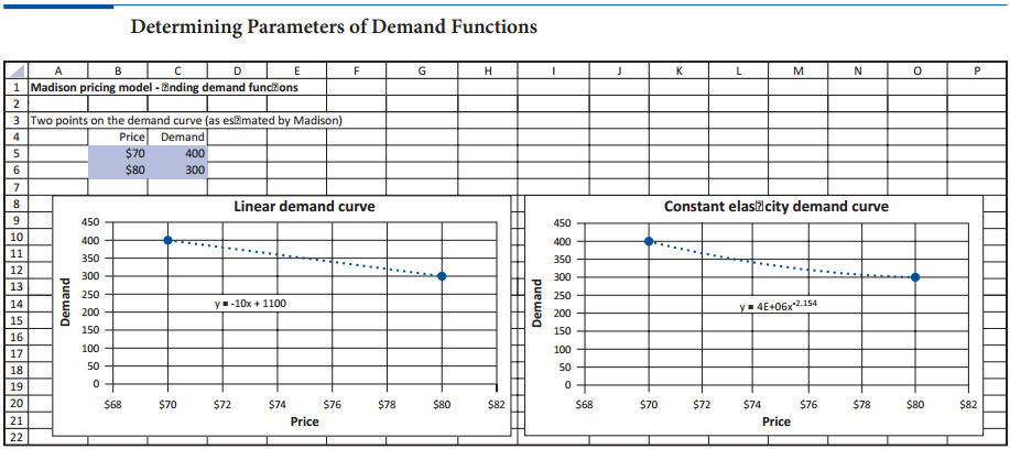
In Example 7.1, two points on the demand curve were given (Figure 7.11).a. Suppose three additional points are estimated by Madison: (1) demand of 460 when price is $65, (2) demand of 355 when price is $75, and (3) demand of 275 when price is $85. With these new points and the
In Example 7.1, one demand function is linear and the other is called a constant elasticity demand function. Using data tables, show that the price elasticity in the linear demand function is not constant in price, and show that the price elasticity is constant in the constant elasticity demand
In the pricing model in Example 7.1 with the constant elasticity demand function, the assumption is that all units demanded are sold. Suppose the company has the capacity to produce only 200 units. If demand is less than capacity, all of demand is sold. If demand is greater than or equal to
Continuing the previous problem, create a two-way data table similar to the one-way data table in Figure?7.11. This time, however, allow price to vary down a column and allow the capacity to vary across a row. Each cell of the data table should capture the corresponding profit. Explain how the
Continuing Problem 3 in a slightly different direction, create a two-way SolverTable where the inputs are the elasticity and the production capacity, and the outputs are the optimal price and the optimal profit. Discuss your findings.Data from Problem 3:In the pricing model in Example 7.1 with the
In the exchange rate model in Example 7.2, suppose the company continues to manufacture its product in the United States, but now it sells its product in the United States, the United Kingdom, and possibly other countries. The company can independently set its price in each country where it sells.
The preceding problem indicates how fewer alternatives can cause total cost to increase. This problem indicates the opposite. Starting with the solution to the advertising selection problem in Example 7.6, add a new show, “The View,” which appeals primarily to women. Use the following constants
Change the exchange rate model in Example 7.2 slightly so that the company is now a UK manufacturing company producing for a U.S. market. Assume that the unit cost is now £75, the demand function has the same parameters as before (although the price for this demand function is now in dollars),
In the exchange rate model in Example 7.2, we found that the optimal unit revenue, when converted to dollars, is $85.71. Now change the problem so that the company is selling in Japan, not the United Kingdom. Assume that the exchange rate is 0.00965 ($/¥) and that the constant in the demand
In the complementary-product pricing model in Example 7.3, the elasticity of demand for suits is currently -2.5. Use SolverTable to see how the optimal price of suits and the optimal profit vary as the elasticity varies from -2.7 to -1.8 in increments of 0.1. Are the results intuitive? Explain.
Continuing Problem 6, suppose the company is selling in the United States, the United Kingdom, and Japan. Assume the unit production cost is $50, and the exchange rates are 1.66 ($/£) and 0.00965 ($/¥). Each country has its own constant elasticity demand function. The parameters for the United
In the complementary-product pricing model in Example 7.3, we have assumed that the profit per unit from shirts and ties is given. Presumably this is because the prices of these products have already been set. Change the model so that the company must determine the prices of shirts and ties, as
Continuing the previous problem (the model in part a) one step further, assume that shirts and ties are also complementary. Specifically, assume that each time a shirt is purchased (and is not accompanied by a suit purchase), 1.3 ties, on average and regardless of the price of ties, are also
In estimating the advertising response function in Example 7.5, we indicated that the sum of squared prediction errors or RMSE could be used as the objective, and we used RMSE. Try using the sum of squared prediction errors instead. Does Solver find the same solution as in the example? Try running
The best-fitting advertising response function in Example 7.5 fits the observed data. This is because we rigged the observed data to fall close to a curve of the form in Equation (7.4). See what happens when one of the observed points is an outlier—that is, it doesn’t fit
The advertising response function in Equation (7.4) is only one of several non-linear functions that could be used to get the same “increasing at a decreasing rate” behavior in Example 7.5. Another possibility is the function f (n) = anb, where a and b are again constants to be
By the time you are reading this, the 2013–2014 NBA season will have finished, and the results should be available at http://www.basketball-reference.com/leagues/NBA_2014_games.html. Do whatever it takes to get the data into Excel in the format of this example. Then, use Solver to find the
The method for rating teams in Example 7.8 is based on actual and predicted point spreads. This method can be biased if some teams run up the score in a few games. An alternative possibility is to base the ratings only on wins and losses. For each game, you observe whether the home team wins. Then
In the model in Example 7.9, stock 2 is not in the optimal portfolio. Use SolverTable to see whether it ever enters the optimal portfolio as its correlations with stocks 1 and 3 vary. Specifically, use a two-way SolverTable with two inputs, the correlations between stock 2 and stocks 1 and 3, each
The stocks in Example 7.9 are all positively correlated. What happens when they are negatively correlated? Answer for each of the following scenarios. In each case, two of the three correlations are the negatives of their original values. Discuss the differences between the optimal portfolios
In many cases, the portfolio return is at least approximately normally distributed. Then Excel’s NORMDIST function can be used to calculate the probability that the portfolio return is negative. The relevant formula is =NORMDIST(0,mean,stdev,1), where mean and stdev are the
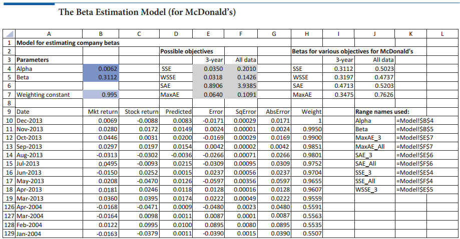
Given the data in the file Stock Beta.xlsx, estimate the beta (and alpha) for Microsoft (MSFT). Do this for each criterion and each period of time to obtain a table analogous to that in the top right of Figure 7.49. What do you conclude about Microsoft?Figure 7.49: The Beta Estimation
Solve the previous problem, but analyze GE instead of Microsoft.Data from Previous Problem:Given the data in the file Stock Beta.xlsx, estimate the beta (and alpha) for Microsoft (MSFT). Do this for each criterion and each period of time to obtain a table analogous to that in the top
Suppose Ford currently sells 250,000 Ford Mustangs annually. The unit cost of a Mustang, including the delivery cost to a dealer, is $16,000. The current Mustang price is $20,000, and the current elasticity of demand for the Mustang is –1.5.a. Determine a profit-maximizing price for a

Showing 1900 - 2000 of 2541

First
12
13
14
15
16
17
18
19
20
21
22
23
24
25
26

Step by Step Answers

Services

Sitemap
Fun
Definitions
Become Tutor
Used Textbooks
Study Help Categories
Recent Questions
Expert Questions
Campus Wear
Sell Your Books

Company Info

Security
Copyrights
Privacy Policy
Terms & Conditions
SolutionInn Fee
Scholarship
Online Quiz
Give Feedback, Get Rewards

Get In Touch

About Us
Contact Us
Career
Jobs
FAQ
Student Discount
Campus Ambassador

Secure Payment

Download Our App

© 2026 SolutionInn. All Rights Reserved