New Semester Started Get 50% OFF Study Help! --h --m --s Claim Now

Question Answers

Textbooks

Find textbooks, questions and answers

Oops, something went wrong!

Change your search query and then try again

Result Not Found

Books FREE
Study Help
Tutors
AI Study Planner NEW
Sell Books

Search
Sign In
Register

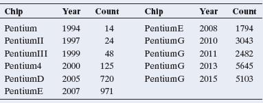
study help
business
statistics alive

Statistics The Art And Science Of Learning From Data 4th Global Edition Alan Agresti, Christine A. Franklin, Bernhard Klingenberg - Solutions

12.99 Multiple choice: Income and height University of Rochester economist Steven Landsburg surveyed economic studies in England and the United States that showed a positive correlation between height and income.The article stated that in the United States each one-inch increase in height was worth
12.98 Multiple choice: Regress x on y The regression of y on x has a prediction equation of yn = -2.0 + 5.0x and a correlation of 0.3. Then, the regression of x on ya. also has a correlation of 0.3.b. could have a negative slope.c. has r2 = 20.3.d. = 1> 1 -2.0 + 5.0y2.
12.97 Multiple choice: Slope and correlation The slope of the least squares regression equation and the correlation are similar in the sense thata. They both must fall between -1 and +1.b. They both describe the strength of association.c. Their squares both have proportional reduction in error
12.96 Multiple choice: Correlation invalid The correlation is appropriate for describing association between two quantitative variablesa. Even when different people measure the variables using different units (e.g., kilograms and pounds).b. When the relationship is highly nonlinear.c. When the
12.95 Multiple choice: Interpret r One can interpret r = 0.30 or the corresponding r2 = 0.09 as follows:a. A 30% reduction in error occurs in using x to predict y.b. A 9% reduction in error occurs in using x to predict y compared to using y to predict y.c. 9% of the time yn = y.d. y changes 0.3
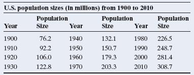
12.94 Population growth Exercise 12.57 about U.S. population growth showed a predicted growth rate of 13% per decade.a. Show that this is equivalent to a 1.23% predicted growth per year.b. Explain why the predicted U.S. population size (in millions) x years after 1900 is 81.137(1.0123)x
12.93 Decrease in home values A Freddie Mac quarterly statement(May 2010) reported that U.S. home sales for one of the central regions (including Illinois, Indiana, Ohio, and Wisconsin) have shown that home values decreased by 3.4% in the last previous year. What if someone interprets this
12.92 Lots of standard deviations Explain carefully the interpretations of the standard deviations (a) sy, (b) sx, (c) residual standard deviation s, and (d) se of slope estimate b.
12.91 Assumptions fail? Refer to the previous exercise. In view of these assumptions, indicate why such a model would or would not be good in the following situations:a. x = year (from 1900 to 2005), y = percentage unemployed workers in the United States. (Hint:Does y continually tend to increase
12.90 Assumptions What assumptions are needed to use the linear regression model to (a) obtain a meaningful fit that represents the true relationship well and (b) to make inferences about the relationship. For partb, which assumption is least critical?
12.89 df for t tests in regression In regression modeling, for t tests about regression parameters, df = n - number of parameters in equation for the mean.a. Explain why df = n - 2 for the model my = a + bx.b. Chapter 8 discussed how to estimate a single mean m.Treating this as the parameter in a
12.88 All models are wrong The statistician George Box, who had an illustrious academic career at the University of Wisconsin, is often quoted as saying, “All models are wrong, but some models are useful.” Why do you think that, in practice,a. All models are wrong?b. Some models are not useful?
12.87 Dollars and pounds Annual income, in dollars, was the response variable in a regression analysis. For a British version of a written report about the analysis, all responses were converted to British pounds sterling(£1 equaled $2.00 when this was done).a. How, if at all, does the slope of
12.86 Mileage and weight Explain why the correlation between x = weight of a car and y = mileage of a car is likely to be smaller if we use a random sample of sports cars than if we use a random sample of all cars.
12.85 Height and weight Suppose the correlation between height and weight is 0.50 for a sample of males in elementary school and 0.50 for a sample of males in middle school.If we combine the samples, explain why the correlation will probably be larger than 0.50.
12.84 Regression toward the mean paradox Does regression toward the mean imply that, over many generations, there are fewer and fewer very short people and very tall people? Explain your reasoning. (Hint: What happens if you look backward in time in doing the regressions?)
12.83 Sports and regression One of your relatives is a big sports fan but has never taken a statistics course. Explain how you could describe the concept of regression toward the mean in terms of a sports application, without using technical jargon.
12.82 Iraq war and reading newspapers A study by the Readership Institute3 at Northwestern University used survey data to analyze how newspaper reader behavior was influenced by the Iraq war. The response variable was a Reader Behavior Score (RBS), a combined measure summarizing newspaper use
12.81 Football point spreads For a football game in the National Football League, let y = difference between number of points scored by the home team and the away team (so, y 7 0 if the home team wins). Let x be the predicted difference according to the Las Vegas betting spread. For the 768 NFL
12.80 Female athletes’ speed For the High School Female Athletes data set on the book’s website, conduct a regression analysis using the time for the 40-yard dash as the response variable and weight as the explanatory variable.Prepare a two-page report, indicating why you conducted each
12.79 GPA and TV watching Using software with the FL Student Survey data file on the book’s website, conduct regression analyses relating y = high school GPA and x = hours of TV watching. Prepare a two-page report, showing descriptive and inferential methods for analyzing the relationship.
12.78 Runs and hits Refer to the previous exercise. Conduct a regression analysis of y = RUNS and x = HIT. Does a straight-line regression model seem appropriate? Prepare a reporta. Using graphical ways of portraying the individual variables and their relationship.b. Interpreting descriptive
12.77 Softball data The Softball data file on the book’s website contains the records of a University of Georgia coed intramural softball team for 277 games over a 20-year period. (The players changed, but the team continued.)The variables include, for each game, the team’s number of runs
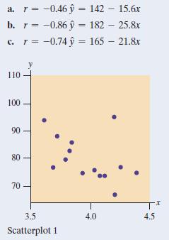
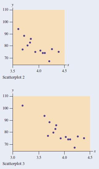
12.76 Match the scatterplot Match each of the following scatterplots to the description of its regression and correlation.The plots are the same except for a single point.Justify your answer for each scatterplot. (Hint: Think about the possible effect of an outlier in the x-direction and an outlier
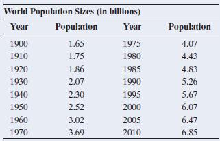
12.75 World population growth The table shows the world population size (in billions) since 1900.a. Let x denote the number of years since 1900. The exponential regression model fitted to y = population size and x gives yn = 1.424 * 1.014x. Show that the predicted population sizes are 1.42 billion
12.74 Florida population The population size of Florida(in thousands) since 1830 has followed approximately the exponential regression yn = 4611.0362x. Here, x = year - 1830 (so, x = 0 for 1830 and x = 170 for the year 2000).a. What has been the approximate rate of growth per year?b. Find the
12.73 Savings growth You invest €2000 in an account having an interest rate such that your principal doubles every 10 years.a. How much money would you have after 60 years?b. If you were still alive after 90 years, show that you would be a millionaire.c. Give the equation relating y = principal
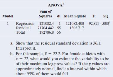
12.72 Leg press ANOVA The analysis in the previous exercise has the ANOVA table shown.a. For those female athletes who had maximum bench press equal to the sample mean of 80 pounds, what is the estimated standard deviation of their maximum leg press values?b. Assuming that maximum leg press has a
12.71 Bench press predicting leg press For the study of high school female athletes, when we use x = maximum bench press (maxBP) to predict y = maximum leg press (maxLP), we get the results that follow. The sample mean of maxBP was 80. Regression Equation maxLP (lbs) 174.0 +2.216 maxBP (lbs) Term
12.70 Exercise and college GPA For the Georgia Student Survey file on the book’s website, let y = exercise and x = college GPA.a. Construct a scatterplot. Identify an outlier that could influence the regression line. What would you expect its effect to be on the slope and the correlation?b. Fit
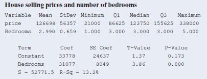
12.69 Types of variability Refer to the previous two exercises.a. Explain the difference between the residual standard deviation of 52,771.5 and the standard deviation of 56,357 reported for the selling prices.b. Since they’re not much different, explain why this means that number of bedrooms is
12.68 Bedrooms affect price? Refer to the previous exercise.a. Explain what the regression parameter b means in this context.b. Construct and interpret a 95% confidence interval for b.c. Use the result of part b to form a 95% confidence interval for the difference in the mean selling prices for
12.67 Bedroom residuals For the House Selling Prices FL data set on the book’s website, when we regress y = selling price (in dollars) on x = number of bedrooms, we get the results shown in the printout.a. One home with three bedrooms sold for $338,000.Find the residual and interpret.b. The home
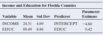
12.66 Income and education in Florida The FL Crime data file on the book’s website contains data for all counties in Florida on y = median annual income (thousands of dollars)for residents of the county and x = percentage of residents with at least a high school education. The table shows some
12.65 Tall people Do very tall parents tend to have children who are even taller, or tall but not as tall as they are?Explain, identifying the response and explanatory variables and the role of regression toward the mean.
12.64 Stem cells In the article, “Variation in cancer risk among tissues can be explained by the number of stem cell divisions” (Tomasetti and Vogelstein, Science, vol.47, 2015), the authors stated: “A linear correlation equal to 0.804 suggests that 65% of the differences in cancer risk among
12.63 Theory exam–practical exam correlation A report summarizing scores for students appearing in a theory examination x and a practical examination y states that x = 270, y = 360, sx = 60, sy = 80, and r = 0.60.a. Find the slope of the regression line, based on its connection with the
12.62 Academic performance and participation in extracurricular activities Let y = grade point average (GPA) and x =number of times a student has participated in extracurricular activities, measured for all students at a university.Explain the mean and variability about the mean aspects of the
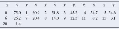
12.61 More leaf litter Refer to the previous exercise.a. The correlation equals -0.890 between x and y and-0.997 between x and log(y). What does this tell you about which model is more appropriate?b. The half-life is the time for the weight remaining to be one-half of the original weight. Use the
12.60 Leaf litter decay Ecologists believe that organic material decays over time according to an exponential decay model.This is the case 0 6 b 6 1 in the exponential regression model, for which my decreases over time. The rate of decay is determined by a number of factors, including composition
12.59 Age and death rate Let x denote a person’s age and let y be the death rate, measured as the number of deaths per thousand individuals of a fixed age within a period of a year. For women in a European country, these variables follow approximately the equation yn = 0.3411.0812x.a. Interpret
12.58 Future shock Refer to the previous exercise, for which predicted population growth was 14.18% per decade.Suppose the growth rate is now 15% per decade. Explain why the population size will (a) double after five decades,(b) quadruple after 100 years (10 decades), and (c) be 16 times its
12.57 U.S. population growth The table shows the approximate U.S. population size (in millions) at 10-year intervals beginning in 1900. Let x denote the number of decades since 1900. That is, 1900 is x = 0, 1910 is x = 1, and so forth. The exponential regression model fitted to y = population size
12.56 Moore’s law today The following data show the number of components (per square inch, in millions) being packed on a Pentium-type chip, for years 1994 to 2015.Let x be the number of years since 1994 (e.g., x = 0 for 1994, x = 3 for 1997, …, x = 21 for 2015) and let y be the number of
12.55 Growth by year versus decade It is expected that the female population in a city will double in two decades.a. Explain why this is possible for a growth rate of 3.6% a year. (Hint: What does 11.036220 equal?)b. You might think that a growth rate of 5% a year would result in 100% growth (i.e.
12.54 Savings grow exponentially You invest $100 in a savings account with interest compounded annually at 10%.a. How much money does the account have after one year?b. How much money does the account have after five years?c. How much money does the account have after x years?d. How many years does
12.53 Cell phone ANOVA Report the ANOVA table for the previous exercise.a. Verify that total SS = residual SS + regression SS. Explain what each of the three sums of squares represent.b. Find the estimated residual standard deviation of y.Interpret it.c. Find the sample standard deviation sy of y
12.52 Predicting cell phone weight Refer to the cell phone data file on the book’s website. Regress y = weight on x = capacity of battery, excluding the outlier (phone no. 70).a. Stating the necessary assumptions, find a 95% confidence interval for the mean weight of cell phones with a battery
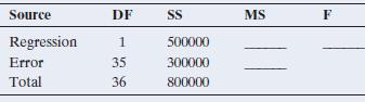
12.51 Understanding an ANOVA table For a random sample of Indian states, the ANOVA table shown refers to hypothetical data on x = tax revenue in Indian rupees and y = agricultural subsidies in Indian rupees.a. Fill in the blanks in the table.b. For what hypotheses can the F test statistic be used?
12.50 Assumption violated For prediction intervals, an important inference assumption is a constant standard deviation s of y values at different x values. In practice, the standard deviation often tends to be larger when my is larger.a. Sketch a hypothetical scatterplot for which this happens,
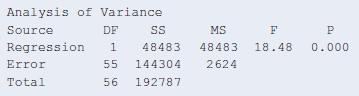
12.49 Variability and F Refer to the previous two exercises.a. In the ANOVA table, show how the Total SS breaks into two parts and explain what each part represents.b. From the ANOVA table, explain why the overall sample standard deviation of y values is sy = 2192787>56 = 58.7. Explain the
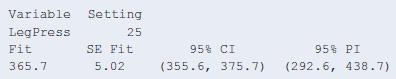
12.48 Predicting leg press Refer to the previous exercise.MINITAB reports the tabulated results for observations at x = 25.a. Show how MINITAB got the “Fit” of 365.7.b. Using the predicted value and se value, explain how MINITAB got the interval listed under “95% CI.”Interpret this
12.47 ANOVA table for leg press Exercise 12.15 referred to an analysis of leg strength for 57 female athletes, with y = maximum leg press and x = number of 200-pound leg presses until fatigue, for which yn = 233.89 + 5.27x.The table shows ANOVA results from SPSS for the regression analysis. ANOVAb
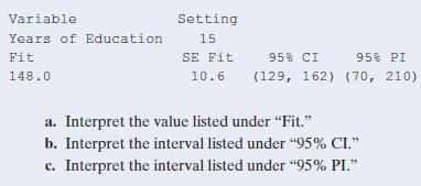
12.46 CI versus PI Using the context of the previous exercise, explain the difference between the purpose of a 95% prediction interval (PI) for an observation and a 95% confidence interval (CI) for the mean of y at a given value of x. Why would you expect the PI to be wider than the CI?
12.45 Predicting annual salary For a random sample of residents from a district in South Carolina, a regression analysis is conducted of y = salary in thousands of dollars and x = years of education. MINITAB reports the tabulated results for observations at x = 15. Variable Years of Education Fit
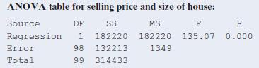
12.44 Predicting house prices The House Selling Prices FL data file on the book’s website has several predictors of house selling prices. The table here shows the ANOVA table for a regression analysis of y = the selling price(in thousands of dollars) and x = the size of house (in thousands of
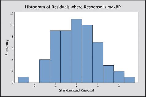
12.43 Bench press residuals The figure is a histogram of the standardized residuals for the regression of maximum bench press on number of 60-pound bench presses for the high school female athletes.a. Which distribution does this figure provide information about?b. What would you conclude based on
12.42 Loves TV and exercise For the Georgia Student Survey file on the book’s website, let y = time exercising and x = time watching TV. One student reported watching TV an average of 180 minutes a day and exercising 60 minutes a day. This person’s residual was 48.8 and the standardized
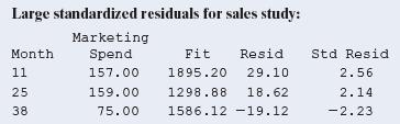
12.41 Poor predicted sales The MINITAB output shows the large standardized residuals for studying sales in thousands of pounds as a response using marketing in thousands of pounds as the explanatory variable.a. Explain how to interpret all the entries in the row of the output for month 11, where
12.40 Correlations for the strong and for the weak Refer to the High School Female Athlete and Male Athlete Strength data files on the book’s website.a. Find the correlation between number of 60-pound bench presses before fatigue and bench press maximum for females and between bench presses
12.39 Violent crime and single-parent families Use software to analyze the U.S. Statewide Crime data file on the book’s website on y = violent crime rate and x = percentage of single parent families.a. Construct a scatterplot. What does it show?b. One point is quite far removed from the others,
12.38 Yale and UConn For which student body do you think the correlation between high school GPA and college GPA would be higher: Yale University or the University of Connecticut? Explain why.
12.37 Food and drink sales The owner of Bertha’s Restaurant is interested in whether an association exists between the amount spent on food and the amount spent on drinks for the restaurant’s customers. She decides to measure each variable for every customer in the next month. Each day she also
12.36 Car weight and mileage The Car Weight and Mileage data file on the book’s website shows the weight and the mileage per gallon of gas of 25 cars of various models.The regression of mileage on weight has r2 = 0.75.Explain how to interpret this in terms of how well you can predict a car’s
12.35 Golf regression In the first round of a golf tournament, five players tied for the lowest round, at 65. The mean score of all players was 75. If the mean score of all players is also 75 in the second round, what does regression toward the mean suggest about how well we can expect the five
12.34 What’s wrong with your stock fund? Last year you looked at all the financial firms that had stock growth funds. You picked the growth fund that had the best performance last year (ranking at the 99th percentile on performance) and invested all your money in it this year.This year, with its
12.33 Was the advertising strategy helpful? Among the 100 different varieties of bread made by a bakery, the marketing manager selected the 10 worst-selling bread types and promoted them through a special advertising strategy. Both the mid-month and the end-month sales had an average of 70 packets
12.32 Placebo helps cholesterol? A clinical trial admits subjects suffering from high cholesterol, who are then randomly assigned to take a drug or a placebo for a 12-week study.For the population, without taking any drug, the correlation between the cholesterol readings at times 12 weeks apart is
12.31 GPA and study time Refer to the association you investigated in Exercise 12.7 between study time and college GPA. Using software or a calculator with the data file you constructed for that exercise,a. Find and interpret the correlation.b. Find and interpret r2. Use the interpretation of r 2
12.30 GPA and TV watching For the Georgia Student Survey data file on the book’s website, the correlation between daily time spent watching TV and college GPA is -0.35.a. Interpret r and r2. Use the interpretation of r2 that(i) refers to the prediction error and (ii) the percent of variability
12.29 GRE score regression toward mean Refer to the previous exercise.a. Predict the verbal GRE score for a student whose math GRE score = 170.b. The correlation is 0.8. Interpret the prediction in part a in terms of regression toward the mean.
12.28 Verbal and math GRE scores All graduate students who attend an Irish university must submit their math and verbal GRE scores. Both the scores have a mean of 150 and a standard deviation of 6.5. The regression equation relating y = verbal GRE score and x = math GRE score is yn = 30 + 0.80x.a.
12.27 Body fat For the Male Athlete Strength data file on the book’s website, the correlation between weight (pounds)and percent body fat (BF%) equals 0.883.a. Interpret the sign and the strength of the correlation.b. Find and interpret r 2.c. If weight were measured instead with metric units,
12.26 Sit-ups and the 40-yard dash Is there a relationship between x = how many sit-ups you can do and y = how fast you can run 40 yards (in seconds)? The MINITAB output of a regression analysis based on the female athlete strength study is shown here.a. Find the predicted time in the 40-yard dash
12.25 Sketch scatterplot Sketch a scatterplot, identifying quadrants relative to the sample means as in Figure 12.2, for which (a) the slope and correlation would be negative and (b) the slope and correlation would be approximately zero.
12.24 When can you compare slopes? Although the slope does not measure association, it is useful for comparing effects for two variables that have the same units. Let x = GDP (thousands of pounds per capita). For predicting y = consumer expenditure, the prediction equation is yn = 3034.89 + 0.52x.
12.23 Euros and thousands of euros If a slope is 1.63 when x = investment in thousands of euros, then what is the slope when x = investment in euros? (Hint: A €1 change has only 1/1000 of the impact of a €1000 change.)
12.22 Battery capacity Refer to the cell phone data set from Exercise 12.9 about various specs of cell phones. Treat the weight of the phone as the response and the capacity of the battery as the explanatory variable. Remove the outlier (phone no. 70).a. Is there evidence for an association between
12.21 GPA and skipping class—revisited Refer to the association you investigated in Exercise 12.8 between skipping class and college GPA. Using software with the data file you constructed, construct a 90% confidence interval for the slope in the population. Interpret.
12.20 GPA and study time—revisited Refer to the association you investigated in Exercise 12.7 between study time and college GPA. Using software with the data file you constructed, conduct a significance test of the hypothesis of independence for the one-sided alternative of a positive population
12.19 Investment and rate of interest. A market research company wants to study the relationship between y = investment(in pounds) and x = rate of interest (in percentage), for a British commercial bank. For the last four months, the observations are as shown in the table. The correlation equals
12.18 CI and two-sided tests correspond Refer to the previous two exercises. Using significance level 0.05, what decision would you make? Explain how that decision is in agreement with whether 0 falls in the confidence interval.Do this for the data for both the boys and the girls.
12.17 More girls are good? Repeat the previous exercise using x = number of daughters the woman had, for which the slope estimate was 0.44 1se = 0.292.
12.16 More boys are bad? A study of 375 women who lived in pre-industrial Finland (by S. Helle et al., Science, vol. 296, p. 1085, 2002), using Finnish church records from 1640 to 1870, found that there was roughly a linear relationship between y = life length (in years) and x = number of sons the
12.15 Strength through leg press The high school female athlete strength study also considered prediction of y = maximum leg press (maxLP) using x = number of 200-pound leg presses (LP200). MINITAB results of a regression analysis are shown.a. Show all steps of a two-sided significance test of the
12.14 House prices in bad part of town Refer to the previous exercise. Of the 100 homes, 25 were in a part of town considered less desirable. For a regression analysis using y = selling price and x = size of house for these 25 homes,a. You plan to test H0: b = 0 against Ha: b 7 0. Explain what H0
12.13 Confidence interval for slope Refer to the previous exercise, which mentioned a confidence interval of (64, 90)for the slope. The 100 houses included in the data set had sizes ranging from 370 square feet to 4,050 square feet.a. Interpret what the confidence interval implies for a one-unit
12.12 Predicting house prices For the House Selling Prices FL data file on the book’s website, MINITAB results of a regression analysis are shown for 100 homes relating y = selling price (in dollars) to x = the size of the house(in square feet).a. Using this output, go through all steps of a
12.11 t-score? A regression analysis is conducted with 32 observations.a. What is the df value for inference about the slope b?b. Which two t test statistic values would give a P-value of 0.10 for testing H0: b = 0 against Ha: b • 0?c. What is the value of the t-score that you multiply the
12.10 Exercise and watching TV For the Georgia Student Survey file on the book’s website, let y = exercise and x = watch TV (minutes per day).a. Construct a scatterplot. Identify an outlier that could have an impact on the fit of the regression model. What would you expect its effect to be on the
12.9 Cell phone specs Refer to the cell phone data set available on the book’s website, which shows various specs of a random sample of cell phones. Engineers would like to analyze how the weight (measured in grams) of a phone depends on the size of the battery, the heaviest component of a cell
12.8 GPA and skipping class Refer to the previous exercise.Now let x = number of classes skipped and y = college GPA.a. Construct a scatterplot. Does the association seem to be positive or negative?b. Find the prediction equation and interpret the y-intercept and slope.c. Find the predicted GPA and
12.7 Study time and college GPA Exercise 3.39 in Chapter 3 showed data collected at the end of an introductory statistics course to investigate the relationship between x = study time per week (average number of hours) and y = college GPA. The table here shows the data for the eight males in the
12.6 Fast food and indigestion Let y = number of times fast food was eaten in the past month and x = number of times indigestion happened in the past month, measured for all students at your school. Explain the mean and variability aspects of the regression model my = a + bx in the context of these
12.5 Ensuring linear relationship In a linear regression model, how does one ensure that the relationship between the dependent variable and the independent variable is linear? Explain.
12.4 Higher income with experience Suppose the regression line my = -10,000 + 9500x models the relationship for the population of working adults in a country between x = experience (in years) and the mean of y = annual income(in US dollars). The conditional distribution of y at each value of x is
12.3 Predicting maximum bench strength in males For the Male Athlete Strength data file on the book’s website, the prediction equation relating y = maximum bench press(maxBP) in kilograms to x = repetitions to fatigue bench press (repBP) is yn = 117.5 + 5.86 x.a. Find the predicted maxBP for a
12.2 Predicting car mileage Refer to the previous exercise.a. Find the predicted mileage for the Toyota Corolla, which weighs 2,590 pounds.b. Find the residual for the Toyota Corolla, which has observed mileage of 38.c. Sketch a graphical representation of the residual in part b.
12.1 Car mileage and weight The Car Weight and Mileage data file on the book’s website shows the weight (in pounds) and mileage (miles per gallon) of 25 different model autos.a. Identify the natural response variable and explanatory variable.b. The regression of mileage on weight has MINITAB
11.90 Conduct a research study using the GSS Go to the GSS codebook at sda.berkeley.edu/GSS. Your instructor will assign a categorical response variable. Conduct a research study in which you find at least two other categorical variables that have both a statistically significant and a practically

Showing 1100 - 1200 of 6613

First
5
6
7
8
9
10
11
12
13
14
15
16
17
18
19
Last

Step by Step Answers

Services

Sitemap
Fun
Definitions
Become Tutor
Used Textbooks
Study Help Categories
Recent Questions
Expert Questions
Campus Wear
Sell Your Books

Company Info

Security
Copyrights
Privacy Policy
Terms & Conditions
SolutionInn Fee
Scholarship
Online Quiz
Give Feedback, Get Rewards

Get In Touch

About Us
Contact Us
Career
Jobs
FAQ
Student Discount
Campus Ambassador

Secure Payment

Download Our App

© 2026 SolutionInn. All Rights Reserved