New Semester Started Get 50% OFF Study Help! --h --m --s Claim Now

Question Answers

Textbooks

Find textbooks, questions and answers

Oops, something went wrong!

Change your search query and then try again

Result Not Found

Books FREE
Study Help
Tutors
AI Study Planner NEW
Sell Books

Search
Sign In
Register

study help
business
statistics alive

Statistics The Art And Science Of Learning From Data 4th Global Edition Alan Agresti, Christine A. Franklin, Bernhard Klingenberg - Solutions

13.92 Logistic slope At the x value where the probability of success is some value p, the line drawn tangent to the logistic regression curve has slope bp11 - p2.a. Explain why the slope is b>4 when p = 0.5.b. Show that the slope is weaker at other p values by evaluating this at p = 0.1, 0.3, 0.7,
13.94 Class data Refer to the data file your class created in Activity 3 in Chapter 1. For variables chosen by your instructor, fit a multiple regression model and conduct descriptive and inferential statistical analyses. Interpret and summarize your findings and prepare to discuss these in class.
13.91 Parabolic regression A regression formula that gives a parabolic shape instead of a straight line for the relationship between two variables is my = a + b1 x + b2 x2.a. Explain why this is a multiple regression model, with x playing the role of x1 and x2 (the square of x) playing the role of
13.90 Simpson’s paradox Let y = death rate and x = average age of residents, measured for each county in Louisiana and in Florida. Draw a hypothetical scatterplot, identifying points for each state, such that the mean death rate is higher in Florida than in Louisiana when x is ignored, but lower
13.89 Indicator for comparing two groups Chapter 10 presented methods for comparing means for two groups.Explain how it’s possible to perform a significance test of equality of two population means as a special case of a regression analysis. (Hint: The regression model then has a single
13.88 R can’t go down The least squares prediction equation provides predicted values yn with the strongest possible correlation with y out of all possible prediction equations of that form. Based on this property, explain why the multiple correlation R cannot decrease when you add a variable to
13.87 Adjusted R2 When we use R2 for a random sample to estimate a population R2, it’s a bit biased. It tends to be a bit too large, especially when n is small. Some software also reports Adjusted R2 = R2 - 5p>[n - 1p + 12]611 - R22, where p = number of predictor variables in the model.This is
13.86 Logistic versus linear For binary response variables, one reason that logistic regression is usually preferred over straight-line regression is that a fixed change in x often has a smaller impact on a probability p when p is near 0 or near 1 than when p is near the middle of its range. Let y
13.85 Multicollinearity For the high school female athletes data file, regress the maximum bench press on weight and percent body fat.a. Show that the F test is statistically significant at the 0.05 significance level.b. Show that the P-values are both larger than 0.35 for testing the individual
13.84 Why an F test? When a model has a very large number of predictors, even when none of them truly have an effect in the population, one or two may look significant in t tests merely by random variation. Explain why performing the F test first can safeguard against getting such false information
13.83 Properties of R2 Using its definition in terms of SS values, explain why R2 = 1 only when all the residuals are 0, and R2 = 0 when each yn = y. Explain what this means in practical terms.
13.82 Lurking variable Give an example of three variables for which you expect b • 0 in the model my = a + bx1 but b1 = 0 in the model my = a + b1 x1 + b2 x2. (Hint: The effect of x1 could be completely due to a lurking variable, x2.)
13.81 Scores for religion You want to include religious affiliation as a predictor in a regression model, using the categories Protestant, Catholic, Jewish, Other. You set up a variable x1 that equals 1 for Protestants, 2 for Catholics, 3 for Jewish, and 4 for Other, using the model my = a + bx1.
13.80 True or false: Slopes For data on y = college GPA, x1 = high school GPA, and x2 = average of mathematics and verbal entrance exam score, we get yn = 2.70 + 0.45x1 for simple regression and yn = 0.3 + 0.40x1 + 0.003x2 for multiple regression. For each of the following statements, indicate
13.79 True or false: Regression For each of the following statements, indicate whether it is true or false. If false, explain why it is false. In regression analysis:a. The estimated coefficient of x1 can be positive in the simple model but negative in a multiple regression model.b. When a model is
13.78 True or false: R and R2 For each of the following statements, indicate whether it is true or false. If false, explain why it is false.a. R2 is always the same as the square of ordinary correlation computed between the values of the response variable and the values yn predicted by the
13.77 Multiple choice: Regression effects Multiple regression is used to model y = college cumulative performance index(CPI) using x1 = high school grade and x2 = average monthly attendance percentage.a. It is possible that the coefficient of x1 is positive in a simple regression but negative in
13.76 Multiple choice: Interpret indicator In the model my = a + b1 x1 + b2 x2, suppose that x1 is an indicator variable for smoking, equalling 1 for smokers and 0 for nonsmokers.a. We set x1 = 0 if we want a predicted mean without knowing if the person is a smoker or not.b. The slope effect of x2
13.75 Multiple Choice: Interpret parameter If yn = 2.4 + 4x1 + 3x2 - 6x3, then controlling for x2 and x3, the change in the estimated mean of y when x1 is increased from 25 to 50a. equals 100.b. equals 0.10.c. Cannot be given—depends on specific values of x2 and x3.d. Must be the same as when we
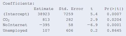
13.74 Unemployment and GDP Refer to Exercise 13.67.When unemployment rate of a country is added as an additional predictor to the model already containing CO2 and percentage of population not using the Internet, we get the following output.a. Interpret the sign of the coefficient for
13.73 Why regression? In 100–200 words, explain to someone who has never studied statistics the purpose of multiple regression and when you would use it to analyze a data set or investigate an issue. Give an example of at least one application of multiple regression. Describe how multiple
13.72 Student data Refer to the FL Student Survey data file on the book’s website. Using software, conduct a regression analysis using y = college GPA and predictors high school GPA and sports (number of weekly hours of physical exercise). Prepare a report, summarizing your graphical analyses,
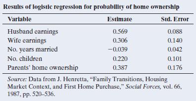
13.71 Factors affecting first home purchase The table summarizes results of a logistic regression model for predictions about first home purchase by young married households.The response variable is whether the subject owns a home 11 = yes, 0 = no2. The explanatory variables are husband’s income,
13.70 AIDS and AZT In a study (reported in the New York Times, February 15, 1991) on the effects of AZT in slowing the development of AIDS symptoms, 338 veterans whose immune systems were beginning to falter after infection with the AIDS virus were randomly assigned either to receive AZT
13.69 Horseshoe crabs and width A study of horseshoe crabs found a logistic regression equation for predicting the probability that a female crab had a male partner nesting nearby by using x = width of the carapace shell of the female crab (in centimeters). The results were Term Coef Constant
13.68 Education and gender in modeling income Consider the relationship between yn = annual income (in thousands of dollars) and x1 = number of years of education by x2 = gender. Many studies in the United States have found that the slope for a regression equation relating y to x1 is larger for men
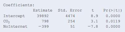
13.67 GDP, CO2, and Internet Consider predicting the per capita GDP (gross domestic product, in thousands of dollars), of a country, using x1 = carbon dioxide emissions per capita (in metric tons) and x2 = percent of country population not using the Internet. Based on data for several countries,
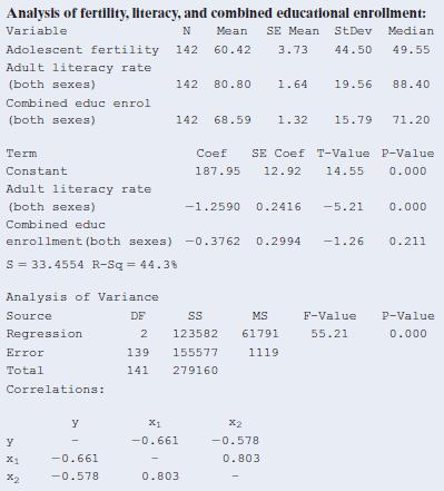
13.66 Significant fertility prediction? Refer to the previous exercise.a. Show how to construct the F statistic for testing H0: b1 = b2 = 0 from the reported mean squares, report its P-value, and interpret.b. If these are the only nations of interest to us for this study, rather than a random
13.65 Modeling fertility For the World Data for Fertility and Literacy data file on the book’s website, a MINITAB printout follows that shows fitting a multiple regression model for y = fertility, x1 = adult literacy rate 1both sexes2, x2 = combined educational enrollment 1both sexes2.Report the
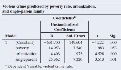
13.64 Effect of poverty on crime Refer to the previous exercise.Now we add x3 = percentage of single-parent families to the model. The SPSS table below shows results.Without x3 in the model, poverty has slope 28.33, and when x3 is added, poverty has slope 14.95. Explain the differences in the
13.63 Violent crime A MINITAB printout is provided from fitting the multiple regression model to U.S. crime data for the 50 states (excluding Washington, D.C.)on y = violent crime rate, x1 = poverty rate, and x2 = percent living in urban areas.a. Predict the violent crime rate for Massachusetts,
13.62 Softball data Refer to the Softball data set on the book’s website. Regress the difference (DIFF) between the number of runs scored by that team and by the other team on the number of hits (HIT) and the number of errors (ERR).a. Report the prediction equation, and interpret the slopes.b.
13.61 Predicting body strength In Chapter 12, we analyzed strength data for a sample of female high school athletes.When we predict the maximum number of pounds the athlete can bench press using the number of times she can do a 60-pound bench press (BP60), we get r2 = 0.643. When we add the number
13.60 House prices This chapter has considered many aspects of regression analysis. Let’s consider several of them at once by using software with the House Selling Prices OR data file on the book’s website to conduct a multiple regression analysis of y = selling price of home, x1 = size of
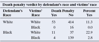
13.58 Death penalty and race The three-dimensional contingency table shown is from a study of the effects of racial characteristics on whether individuals convicted of homicide receive the death penalty. The subjects classified were defendants in indictments involving cases with multiple murders in
13.57 Graduation, gender, and race The U.S. Bureau of the Census lists college graduation numbers by race and gender.The table shows the data for graduating 25-year-olds.College graduation Group Sample Size Graduates White females 31,249 10,781 White males 39,583 10,727 Black females 13,194 2,309
13.56 Many predictors of voting Refer to the previous two exercises. When the explanatory variables are x1 = family income, x2 = number of years of education, and x3 = gender (1 = male, 0 = female), suppose a logistic regression reports Term Coef Constant −2.165 radius 2.585 Term Coef SE Coef
13.55 Equally popular candidates Refer to the previous exercise.a. At which income level is the estimated probability of voting for the Republican candidate equal to 0.50?b. Over what region of income values is the estimated probability of voting for the Republican candidate(i) greater than 0.50
13.54 Voting and income A logistic regression model describes how the probability of voting for the Republican candidate in a presidential election depends on x, the voter’s total family income (in thousands of dollars) in the previous year. The prediction equation for a particular sample is pn
13.53 Cancer prediction (continued) Refer to the previous exercise.For what values of the radius do you estimate that a female has a probability of (a) 0.50, (b) greater than 0.50, and (c) less than 0.50, of having breast cancer?
13.52 Cancer prediction A breast cancer study at a city hospital in New York used logistic regression to predict the probability that a female has breast cancer. One explanatory variable was x = radius of the tumor (in cm). The results are as follows:The quartiles for the radius were Q1 = 1.00, Q2
13.51 Hall of Fame induction Baseball’s highest honor is election to the Hall of Fame. The history of the election process, however, has been filled with controversy and accusations of favoritism. Most recently, there is also the discussion about players who used performance enhancement drugs.
13.50 Income and credit cards Example 12 used logistic regression to estimate the probability of having a travel credit card when x = annual income (in thousands of euros).Show that the estimated probability of having a travel credit card at the income level of €35,000 equals 0.54.
13.49 Comparing revenue An entrepreneur owns two filling stations—one at an inner city location and the other at an interstate exit location. He wants to compare the regressions of y = total daily revenue on x = number of customers who visit the filling station, for total revenue listed on a
13.48 Equal slopes for car prices? Refer to Exercise 13.41, with yn = predicted selling price of used car and x1 = age of car. When equations are fitted separately for U.S. and foreign cars, we get yn = 23,417 - 1,715x1 for U.S. cars and yn = 15,536 - 557x1 for foreign cars.a. In allowing the lines
13.47 House size and garage interact? Refer to the previous exercise.a. Explain what the no interaction assumption means for this model.b. Sketch a hypothetical scatter diagram, showing points identified by garage or no garage, suggesting that there is actually a substantial degree of interaction.
13.46 Houses, size, and garage Use the House Selling Prices OR data file on the book’s website to regress selling price in thousands on house size and whether the house has a garage.a. Report the prediction equation. Find and interpret the equations predicting selling price using house size for
13.45 Predicting pizza sales A chain restaurant that specializes in selling pizza wants to analyze how y = sales for a customer (the total amount spent by a customer on food and beverage, in pounds) depends on the location of the restaurant, which is classified as inner city, suburbia, or at an
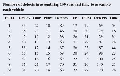
13.44 Quality and productivity The table shows data from 27 automotive plants on y = number of assembly defects per 100 cars and x = time (in hours) to assemble each vehicle.The data are in the Quality and Productivity file on the book’s website.Regression of selling price of house in thousands
13.43 Predict using house size and condition For the House Selling Prices OR data set, when we regress y = selling price (in thousands) on x1 = house size and x2 = condition (1 = Good, 0 = Not Good), we get the results shown.c. Estimate the difference between the mean selling price of homes in good
13.42 Mountain bike prices The Mountain Bike data file on the book’s website shows selling prices for mountains bikes. When y = mountain bike price($) is regressed on x1 = weight of bike (lbs) and x2 = the type of suspension 10 = full, 1 = front end2, yn = 2,741.62 - 53.752x1 - 643.595x2.a.
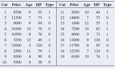
13.41 U.S. and foreign used cars Refer to the used car data file from Exercise 13.11. The prediction equation relating y = selling price of used car (in $) as a function of x1 = age of car and x2 = type of car 11 = US, 0 = Foreign2 is yn = 20,493 - 1,185x1 - 2,379x2.a. Using this equation, find the
13.40 Selling prices level off In the previous exercise, suppose house selling price tends to increase with a straight-line trend for small to medium size lots, but then levels off as lot size gets large, for a fixed value of number of bathrooms.Sketch the pattern you’d expect to get if you
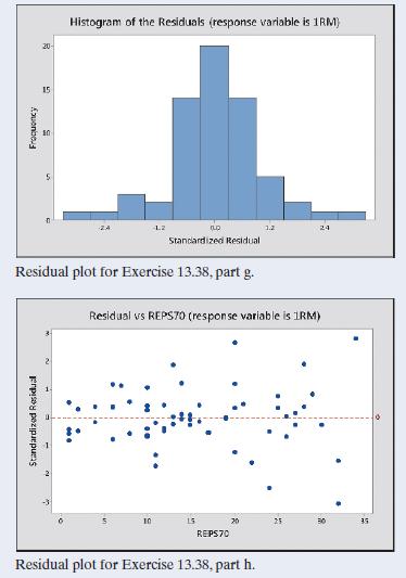
13.39 House prices Use software with the House Selling Prices OR data file on the book’s website to do residual analyses with the multiple regression model for y = house selling price (in thousands), x1 = lot size, and x2 = number of bathrooms.a. Find a histogram of the standardized residuals.
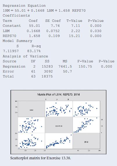
13.38 College athletes The College Athletes data set on the book’s website comes from a study of University of Georgia female athletes. Using the column names from the data set, the response variable 1RM = maximum bench press has explanatory variables LBM = lean body mass (which is weight times 1
13.37 Why inspect residuals? When we use multiple regression, what is the purpose of performing a residual analysis?Why is it better to work with standardized residuals than unstandardized residuals to detect outliers?
13.36 Population growth with time Suppose you fit a straightline regression model to x = time and y = population.Sketch what you would expect to observe for (a) the scatterplot of x and y and (b) a plot of the residuals against the values of time.
13.35 Nonlinear effects of age Suppose you fit a straight-line regression model to y = number of hours worked (excluding time spent on household chores) and x = age of the subject. Values of y in the sample tend to be quite large for young adults and for elderly people, and they tend to be lower
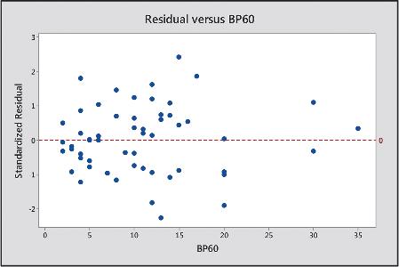
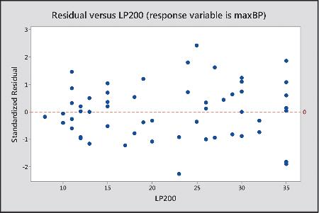
13.34 More residuals for strength Refer to the previous exercise.The following figure is a residual plot for the model relating maximum bench press to LP200 and BP60. It plots the standardized residuals against the values of BP60. Does this plot suggest any irregularities with the model? Explain.
13.33 Strength residuals In Chapter 12, we analyzed strength data for a sample of female high school athletes. The following figure is a residual plot for the multiple regression model relating the maximum number of pounds the athlete could bench press (maxBP) to the number of 60-pound bench
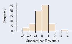
13.32 Body weight residuals Examples 4–7 used multiple regression to predict total body weight of college athletes in terms of height, percent body fat, and age. The following figure shows a histogram of the standardized residuals resulting from fitting this model.a. About which distribution do
13.31 House prices Use software to do further analyses with the multiple regression model of y = selling price of home in thousands, x1 = size of home, and x2 = number of bedrooms, considered in Section 13.1. The data file House Selling Prices OR is on the book’s website.a. Report the F statistic
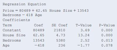
13.30 More predictors for selling price The MINITAB results are shown for predicting selling price using x1 = size of home, x2 = number of bedrooms, and x3 = age.a. State the null hypothesis for an F test, in the context of these variables.b. The F statistic equals 74.23, with P@value =
13.29 Gain in human development Refer to the previous exercise.a. Report the test statistic and P-value for testing H0: b1 = b2 = 0.b. State the alternative hypothesis that is supported by the result in part a.c. Does the result in part a imply that necessarily both literacy rate and daily per
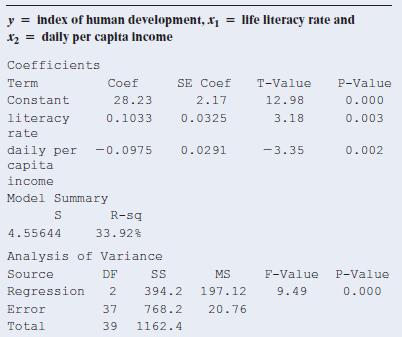
13.28 Regression for human development A study investigated an index of human development in a South American country, which had y = 27.3 and s = 5.5. Two explanatory variables were x1 = literacy rate in percentage(mean = 44.4, s = 22.6) and x2 = daily per capita income in dollars (mean = 56.6, s =
13.27 Predicting restaurant revenue An Italian restaurant keeps monthly records of its total revenue, expenditure on advertising, prices of its own menu items, and the prices of its competitors’menu items.a. Specify notation and formulate a multiple regression equation for predicting the monthly
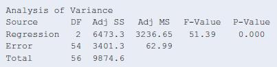
13.26 Any predictive power? Refer to the previous three exercises.a. State and interpret the null hypothesis tested with the F statistic in the ANOVA table given in Exercise 13.23.b. From the F table (Table D), which F statistic value would have a P-value of 0.05 for these data?c. Report the
13.25 Interpret strength variability Refer to the previous two exercises.The sample standard deviation of maxBP was 13.3.The residual standard deviation of maxBP when BP60 and LP200 are predictors in a multiple regression model is 7.9.a. Explain the difference between the interpretations of these
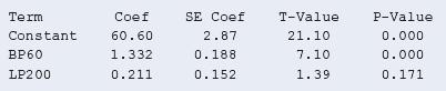
13.24 Leg press uncorrelated with strength? The P-value of 0.17 in part a of the previous exercise suggests that LP200 plausibly had no effect on maxBP once BP60 is in the model. Yet when LP200 is the sole predictor of BP, the correlation is 0.58 and the significance test for its effect has a
13.23 Does leg press help predict body strength?Chapter 12 analyzed strength data for 57 female high school athletes. Upper body strength was summarized by the maximum number of pounds the athlete could bench press (denoted maxBP). This was predicted well by the number of times she could do a
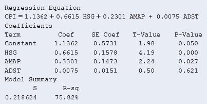
13.22 Variability in college CPI Refer to the previous two exercises.a. Report the residual standard deviation. What does this describe?b. Interpret the residual standard deviation by predicting where approximately 95% of the college CPI fall when high school grade (HSG) = 3.80, average monthly
13.21 Study time helps CPI? Refer to the previous exercise.a. Report and interpret the P-value for testing the hypothesis that the population slope coefficient for study time equals 0.b. Find a 95% confidence interval for the true slope for average daily study time (ADST). Explain how the result is
13.20 Predicting CPI For a random sample of 100 students in a German university, the result of regressing the college cumulative performance index (CPI) on the high school grade (HSG), the average monthly attendance percentage(AMAP) and the average daily study time (ADST) follows.a. Explain in
13.19 Predicting college GPA Using software with the Georgia Student Survey data file from the book’s website, find and interpret the multiple correlation and R2 for the relationship between y = college GPA, x1 = high school GPA, and x2 = study time. Use both interpretations of R2 as the
13.18 Slopes, correlations, and units In Example 2 on y = house selling price, x1 = house size, and x2 = number of bedrooms, yn = 60,102 + 63.0x1 +15,170x2, and R = 0.72.a. Interpret the value of the multiple correlation.b. Suppose house selling prices are changed from dollars to thousands of
13.17 Softball data For the Softball data set on the book’s website, for each game, the variables are a team’s number of runs scored (RUNS), number of hits (HIT), number of errors (ERR), and the difference (DIFF) between the number of runs scored by that team and by the other team, which is the
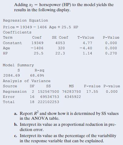
13.16 Price, age, and horsepower In the previous exercise, r2 = 0.66 when age is the predictor and R2 = 0.69 when both age and HP are predictors. Why do you think that the predictions of price don’t improve much when HP is added to the model? (The correlation between HP and price is r = 0.56, and
13.15 Price of used cars For the 19 used cars listed in the Used Cars data file on the book’s website (see also Exercise 13.11), modeling the mean of y = used car price in terms of x1 = age results in r2 = 0.66. Adding x2 = horsepower (HP) to the model yields the results in the following display.
13.14 When does controlling have little effect? Refer to the previous exercise. Height has a similar estimated slope for each of the three models. Why do you think that controlling for % body fat and then age does not change the effect of height much? (Hint: How strongly is height correlated with
13.13 Predicting weight Let’s use multiple regression to predict total body weight (TBW, in pounds) using data from a study of female college athletes. Possible predictors are HGT = height (in inches), %BF = percent body fat, and age. The display shows the correlation matrix for these
13.12 Predicting average monthly visitor satisfaction Refer to Exercise 13.3 about the multiple linear regression of a restaurant’s average monthly visitor satisfaction rating (y) on the monthly food quality score (x1) and the number of visitors in a month (x2). Following is the ANOVA table of
13.11 Used cars The following data (also available from the book’s website) is from a random sample of campus newspaper ads on used cars for sale. Consider the age and horsepower (HP) of a car to predict its selling price.(The variable Type stands for whether the car is from the United States,
13.10 House selling prices Using software with the House Selling Prices OR data file on the book’s website, analyze y = selling price, x1 = house size, and x2 = lot size.a. Construct box plots for each variable and a scatterplot matrix or scatter plots between y and each of x1 and x2.Interpret.b.
13.9 Controlling has an effect The slope of x1 is not the same for multiple linear regression of y on x1 and x2 as compared to simple linear regression of y on x1, where x1 is the only predictor. Explain why you would expect this to be true. Does the statement change when x1 and x2 are uncorrelated?
13.8 Comparable number of bedrooms and house size effects In Example 2, the prediction equation between y = selling price and x1 = house size and x2 = number of bedrooms was yn = 60,102 + 63.0x1 + 15,170x2.a. For fixed number of bedrooms, how much is the house selling price predicted to increase
13.7 The economics of golf The earnings of a PGA Tour golfer are determined by performance in tournaments.A study analyzed tour data to determine the financial return for certain skills of professional golfers. The sample consisted of 393 golfers competing in one or both of the 2002 and 2008
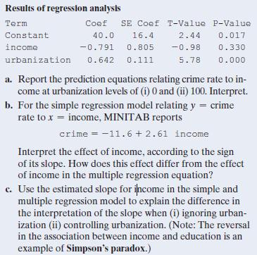
13.6 Crime rate and income Refer to the previous exercise.MINITAB reports the following results for the multiple regression of y = crime rate on x1 = median income(in thousands of dollars) and x2 = urbanization. Results of regression analysis Term Constant income urbanization Coef 40.0 SE Coef
13.5 Does more education cause more crime? The FL Crime data file on the book’s website has data for the 67 counties in Florida on y = crime rate: Annual number of crimes in county per 1000 population x1 = education: Percentage of adults in county with at least a high school education x2 =
13.4 Interpreting slopes on average monthly visitor satisfaction Refer to the previous exercise.a. Explain why setting x2 at a variety of values yields a collection of parallel lines relating yn to x1. What is the value of the slope for those parallel lines?b. Since the slope 0.55 for x1 is larger
13.3 Predicting visitor satisfaction For all the restaurants in a city, the prediction equation for y = average monthly visitor satisfaction rating (range 0–4.0 where 0 =very poor and 4 = very good) and x1 = the monthly food quality score given by the food inspection authority(range 0–4.0 where
13.2 Does study help GPA? For the Georgia Student Survey file on the book’s website, the prediction equation relating y = college GPA to x1 = high school GPA and x2 = study time (hours per day), is yn = 1.13 +0.643x1 + 0.0078x2.a. Find the predicted college GPA of a student who has a high school
13.1 Predicting weight For a study of female college athletes, the prediction equation relating y = total body weight (in pounds) to x1 = height (in inches) and x2 = percent body fat is yn = -121 + 3.50x1 + 1.35x2.a. Find the predicted total body weight for a female athlete at the mean values of 66
12.107 Analyze your data Refer to the data file you created in Activity 3 at the end of Chapter 1. For variables chosen by your instructor, conduct a regression and correlation analysis. Report both descriptive and inferential statistical analyses, interpreting and summarizing your findings and
12.106 Rule of 72 You invest $1000 at 6% compound interest a year. How long does it take until your investment is worth $2000?a. Based on what you know about exponential regression, explain why the answer is the value of x for which 100011.062x = 2000.b. Using the property of logarithms that
12.105 Regression with an error term4 An alternative to the regression formula my = a + bx expresses each y value, rather than the mean of the y values, in terms of x. This approach models an observation on y as y = mean + error = a + bx + e, where the mean my = a + bx and the error = e.The error
12.104 Standard error of slope The formula for the standard error of the sample slope b is se = s>Σ1x - x22, where s is the residual standard deviation.a. Show that the smaller the value of s, the more precisely b estimates b.b. Explain why a small s occurs when the data points show little
12.103 r2 and variances Suppose r2 = 0.30. Since Σ1y - yQ 22 is used in estimating the overall variability of the y values and Σ1y - yn22 is used in estimating the residual variability at any fixed value of x, explain why approximately the estimated variance of the conditional distribution of y
12.102 Why is there regression toward the mean? Refer to the relationship r = 1sx>sy2b between the slope and correlation, which is equivalently sxb = rsy.a. Explain why an increase in x of sx units relates to a change in the predicted value of y of sxb units. (For instance, if sx = 10, it
12.101 Golf club velocity and distance A study about the effect of the swing on putting in golf (by C. M. Craig et al., Nature, vol. 405, 2000, pp. 295–296) showed a very strong linear relationship between y = putting distance and the square of x = club’s impact velocity (r2 is in the range
12.100 True or false The variables y = annual income (thousands of dollars), x1 = number of years of education, and x2 = number of years experience in job are measured for all the employees having city-funded jobs in Knoxville, Tennessee. Suppose that the following regression equations and

Showing 1000 - 1100 of 6613

First
4
5
6
7
8
9
10
11
12
13
14
15
16
17
18
Last

Step by Step Answers

Services

Sitemap
Fun
Definitions
Become Tutor
Used Textbooks
Study Help Categories
Recent Questions
Expert Questions
Campus Wear
Sell Your Books

Company Info

Security
Copyrights
Privacy Policy
Terms & Conditions
SolutionInn Fee
Scholarship
Online Quiz
Give Feedback, Get Rewards

Get In Touch

About Us
Contact Us
Career
Jobs
FAQ
Student Discount
Campus Ambassador

Secure Payment

Download Our App

© 2026 SolutionInn. All Rights Reserved