New Semester Started Get 50% OFF Study Help! --h --m --s Claim Now

Question Answers

Textbooks

Find textbooks, questions and answers

Oops, something went wrong!

Change your search query and then try again

Result Not Found

Books FREE
Study Help
Tutors
AI Study Planner NEW
Sell Books

Search
Sign In
Register

study help
business
bayesian statistics an introduction

Probability & Statistics For Engineers And Scientists With R 1st Edition Michael Akritas - Solutions

14. A study examined the effect of varying the water/cement ratio (X) on the strength (Y)of concrete that has been aged 28 days.3 Use CS=read.table(”WaCeRat28DayS.txt”, header=T) to read the n = 13 pairs of measurements into the R data frame CS. Copy the data into the R objects x and y by
13. A study was conducted to determine the relation between the (easier to measure) conductivity (μS/cm) of surface water and water in the sediment at the bank of a river.2 The summary statistics for 10 pairs of surface (X)and sediment (Y) conductivity measurements are 1Xi = 3728, 1 Yi = 5421, 1
12. In the parametrization μY|X(x) = α1+β1x of the simple linear regression model, μY|X(0) = α1 and !μY|X(0) = !α1. Use this fact and the formula for the (1 − α)100% CI for μY|X(x) to give the formula for the (1 − α)100% CI for α1.
11. To determine the probability that a certain component lasts more than 350 hours in operation, a random sample of 37 components was tested. Of these, 24 lasted longer than 350 hours.(a) Construct a 95% CI for the probability, p, that a randomly selected component lasts more than 350 hours.(b) A
10. A health magazine conducted a survey on the drinking habits of young adult (ages 21–35) US citizens. On the question “Do you drink beer, wine, or hard liquor each week?” 985 of the 1516 adults interviewed responded“yes.”(a) Find a 95% confidence interval for the proportion, p, of
9. In making plans for an executive traveler’s club, an airline would like to estimate the proportion of its current customers who would qualify for membership. A random sample of 500 customers yielded 40 who would qualify.(a) Construct a 95% CI for the population proportion, p, of customers who
8. Copy the Old Faithful geyser’s eruption durations data into the R object ed with the command ed=faithful$eruptions, and use R commands to complete the following parts.(a) Construct a 95% CI for the mean eruption duration.(b) Construct a 95% CI for the median eruption duration.(c) Construct a
7. Fifty newly manufactured items are examined and the number of scratches per item are recorded. The resulting frequencies of the number of scratches is:Number of scratches per item 0 1 2 3 4 Observed frequency 4 12 11 14 9 Assume that the number of scratches per item is a Poisson(λ) random
6. The data file SolarIntensAuData.txt contains n = 40 solar intensity measurements (watts/m2) on different days at a location in southern Australia. Import the data into the R data frame si, copy the data into the R object x by x=si$SI, and use R commands to complete the following parts.(a)
5. The data file OzoneData.txt contains n = 14 ozone measurements (Dobson units) taken from the lower stratosphere, between 9 and 12 miles (15 and 20 km).Import the data into the R data frame oz, copy the data into the R object x by x=oz$OzoneData, and use R commands to complete the following
4. Refer to Exercises 1 and 2.(a) For the data in Exercise 1, find the confidence level of the CIs (36.86, 50.59) and (36.75, 57.16) for the population median distance.(b) For the data in Exercise 2, find the confidence level of the CI (418, 832) for the population median histamine content.
3. For a randomsample of 50measurements of the breaking strength of cotton threads, X = 210 grams and S = 18 grams.(a) Obtain an 80% CI for the true mean breaking strength.What assumptions, if any, are needed for the validity of the CI? (b) Would the 90% CI be wider than the 80% CI constructed in
2. Analysis of the venom of 7 eight-day-old worker bees yielded the following observations on histamine content in nanograms: 649, 832, 418, 530, 384, 899, 755.(a) Construct by hand a 90% CI for the true mean histamine content for all worker bees of this age. What assumptions, if any, are needed
1. A question relating to a study of the echolocation system for bats is how far apart the bat and an insect are when the bat first senses the insect. The technical problems for measuring this are complex and so only n = 11 data points were obtained (in dm):x 57.16, 48.42, 46.84, 19.62, 41.72,
An optical firm purchases glass to be ground into lenses. As it is important that the various pieces of glass have nearly the same index of refraction, the firm is interested in controlling the variability. A simple random sample of size n = 20 measurements yields S2 = (1.2)10−4. From previous
Let X1, . . . ,X25 be a sample from a continuous population. Find the confidence level of the following CI for the median:X(8),X(18)0.
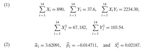
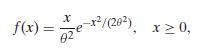
The following summary statistics and least squares estimators were obtained using n = 14 data points on Y= propagation velocity of an ultrasonic stress wave through a substance and X= tensile strength of the substance:A scatterplot for this data does not indicate violation of the assumptions for
Can changes in Gross Domestic Product (GDP) be predicted from changes in the unemployment rate? Quarterly data on changes in unemployment rate (X)and percent change in GDP (Y), from 1949 to 1972, are given in the data file GdpUemp49-72.txt.1 Assuming the simple linear regression model is a
In a low-impact car crash experiment, similar to that described in Example 6.3-4, 18 of 30 cars sustained no visible damage. Construct a 95% CI for the true value of p, the probability that a car of this type will sustain no visible damage in such a low-impact crash.
A random sample of n = 56 cotton pieces gave average percent elongation of X = 8.17 and a sample standard deviation of S = 1.42. Construct a 95% CI for μ, the population mean percent elongation.
The Charpy impact test, developed by French scientist George Charpy, determines the amount of energy, in joules, absorbed by a material during fracture. (Fracture is induced by one blow from a swinging pendulum, under standardized conditions. The test was pivotal in understanding the fracture
2. Let X1, . . . ,X10 be a random sample from a population with mean μ and variance σ2, and Y1, . . . ,Y10 be a random sample from another population with mean also equal to μ and variance 4σ2. The two samples are independent.(a) Show that for any α, 0 ≤ α ≤ 1, !μ = αX +(1−α)Y is
1. Let X1, . . . ,Xn be a random sample from the uniform(0,θ) distribution, and let!θ1 = 2X and!θ2 = X(n), that is, the largest order statistic, be estimators for θ. It is given that the mean and variance of!θ2 are(a) Give an expression for the bias of each of the two estimators. Are they
Simple random vs stratified sampling. Facilities A and B account for 60% and 40%, respectively, of the production of a certain electronic component. The components from the two facilities are shipped to a packaging location where they are mixed and packaged. A sample of size 100 will be used to
Use da=read.table(”TreeAgeDiamSugarMaple.txt”, header=T) to read the data on the diameter (in millimeters)and age (in years) of n = 27 sugar maple trees into the R data frame da. Copy the data into the R objects x and y by x=da$Diamet; y=da$Age, and use R commands to complete the following.(a)
12. Use sm=read.table(”StrengthMoE.txt”, header=T) to read the data on cement’s modulus of elasticity and strength into the R data frame sm. Copy the data into the R objects x and y by x=sm$MoE and y=sm$Strength, and use R commands to complete the following.(a) Construct a scatterplot of the
11. Manatees are large, gentle sea creatures that live along the Florida coast. Many manatees are killed or injured by powerboats. Below are data on powerboat registrations(in thousands) and the number of manatees killed by boats in Florida for four different years between 2001 and 2004:Number of
10. A study was conducted to examine the effects of NaPO4, measured in parts per million (ppm), on the corrosion rate of iron.3 The summary statistics corresponding to 11 data points, where the NaPO4 concentrat 1ions ranged from 2.50 ppm to 55.00 ppm, are as follows: ni=1 xi = 263.53, 1ni=1 yi =
9. Plumbing suppliers typically ship packages of plumbing supplies containing many different combinations of item such as pipes, sealants, and drains. Almost invariably a shipment contains one or more incorrectly filled items:a part may be defective, missing, not the type ordered, etc. In this
8. Let X1, . . . ,Xn be a random sample from the uniform(0, θ) distribution. Use the R command set.seed(3333); x=runif(20, 0, 10) to generate a random sample X1, . . . ,X20 from the uniform(0, 10) distribution, and store it into the R object x.(a) Give the method of moments estimate of θ and the
7. A company manufacturing bike helmets wants to estimate the proportion p of helmets with a certain type of flaw. They decide to keep inspecting helmets until they find r = 5 flawed ones. Let X denote the number of helmets that were not flawed among those examined.(a) Write the log-likelihood
6. Answer the following questions.(a) Let X1, . . . ,Xn be iid Poisson(λ). Find the maximum likelihood estimator of λ.(b) The numbers of surface imperfections for a random sample of 50 metal plates are summarized in the following table:Assuming that the imperfection counts have the Poisson(λ)
5. Answer the following questions.(a) Let X ∼ Bin(n, p). Find the method of moments estimator of p. Is it unbiased?(b) To determine the probability p that a certain component lasts more than 350 hours in operation, a random sample of 37 components was tested. Of these, 24 lasted more than 350
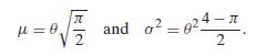
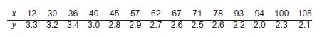
4. The probability density function of the Rayleigh distribution iswhere θ is a positive-valued parameter. It is known that the mean and variance of the Rayleigh distribution areLet X1, . . . ,Xn be a random sample from a Rayleigh distribution.(a) Construct the method of moments estimator of θ.
3. The life spans, in hours, of a random sample of 25 electronic components yield sample mean X = 113.5 hours and sample variance S2 = 1205.55 hours2. Using the method of moments, fit the gamma(α, β) model to this data. (Hint. The mean and variance of the gamma(α, β)distribution are given in
2. Use t=read.table(”RobotReactTime.txt”, header=T);t1=t$Time[t$Robot==1] to import the data on robot reaction times to simulated malfunctions, and copy the reaction times of Robot 1 into the R object t1.(a) Follow the approach of Example 6.3-3 to fit the Weibull(α, β) model to the data in
1. Let X1, . . . ,Xn be iid exponential(λ). Find the method of moments estimator of λ. Is it unbiased?
Use R commands and the n = 153 measurements (taken in New York from May to September 1973) on solar radiation (lang) and ozone level (ppb) from the R data set airquality to complete the following parts.(a) Use the method of LS to fit the simple linear regression model to this data set.(b) Construct
Consider the following data on Y = propagation velocity of an ultrasonic stresswave through a substance and X = tensile strength of substance.(a) Use the method of LS to fit the simple linear regression model to this data.(b) Obtain the error sum of squares and the LSE of the intrinsic error
(a) Let X1, . . . ,Xn be iid uniform(0, θ). Find the maximum likelihood estimator of θ.(b) The waiting times for a random sample of n = 10 passengers of a New York commuter train are: 3.45, 8.63, 8.54, 2.59, 2.56, 4.44, 1.80, 2.80, 7.32, 6.97.Assuming that the waiting times have the uniform(0,
Let x1, . . . , xn be the waiting times for a random sample of n customers of a certain bank. Use the method of maximum likelihood to fit the exponential(λ) model to this data set.
Car manufacturers often advertise damage results from low-impact crash experiments.In an experiment crashing n = 20 randomly selected cars of a certain type against a wall at 5 mph, X = 12 cars sustain no visible damage. Find the MLE of the probability, p, that a car of this type will sustain no
The life spans, in hours, of a random sample of 25 electronic components yield sample mean X = 113.5 hours and sample variance S2 = 1205.55 hours2. Use the method of moments approach to fit theWeibull(α, β) model.
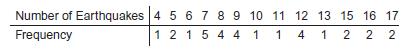
(a) Let X1, . . . ,Xn be iid Poisson(λ). Find the method of moments estimator of λ.Is it unbiased?(b) The weekly counts of earthquakes in North America for 30 consecutive weeks are summarized in the following table:Assuming that the earthquake counts have the Poisson(λ) distribution, compute the
Let X1, . . . ,Xn be a simple random sample taken from some population. Use the method of moments approach to fit the following models to the data:(a) The population distribution of the Xi is uniform(0, θ).(b) The population distribution of the Xi is uniform(α, β).
10. Use cs=read.table(”Concr.Strength.1s.Data.txt”, header=T); x=cs$Str to store the data set2 consisting of 28-day compressive-strength measurements of concrete cylinders using water/cement ratio 0.4 into the R object x.(a) Use the commands given in Section 3.5.2 to produce a normal Q-Q plot
9. Use the R command set.seed=1111; x=rnorm(50, 11, 4) to generate a simple random sample of 50 observations from a N(11, 16) population and store it in the R object x.(a) Give the true (population) values of P(12 < X ≤ 16)and of the 15th, 25th, 55th, and 95th percentiles.(b) Give the
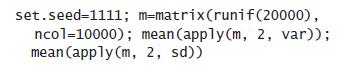
8. The R commandsgenerate 10,000 samples of size n = 2 from the uniform(0, 1) distribution (each column of the matrix m is a sample of size 2), compute the sample variance from each sample, average the 10,000 variances, and do the same for the sample standard deviations.(a) Compare the average of
7. The fat content measurements of a random sample of 6 jugs of 2% lowfat milk jugs of a certain brand are 2.08, 2.10, 1.81, 1.98, 1.91, 2.06.(a) Give the model-free estimate of the proportion of milk jugs having a fat content measurement of 2.05 or more.(b) Assume the fat content measurements are
6. To estimate the proportion p1 of male voters who are in favor of expanding the use of solar energy, take a random sample of size m and set X for the number in favor.To estimate the corresponding proportion p2 of female voters, take an independent random sample of size n and set Y for the number
5. In Example 6.3-1 it is shown that if X1, . . . ,Xn is a random sample from the uniform(0, θ) distribution, the method of moments estimator of θ is!θ = 2X. Give the standard error of!θ . Is!θ unbiased?
4. The financial manager of a department store chain selected a random sample of 200 of its credit card customers and found that 136 had incurred an interest charge during the previous year because of an unpaid balance.(a) Specify the population parameter of interest in this study, give the
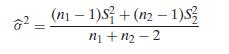
3. In the context of Exercise 2, suppose that the population variance of the maximum penetration is the same for both material types. Call the common population variance σ2, and show thatis an unbiased estimator of σ2. (n-1)+(n-1)S 8 = m+12-2
2. To compare the corrosion-resistance properties of two types of material used in underground pipelines, specimens of both types are buried in soil for a 2-year period and the maximum penetration (in mils) for each specimen is measured. A sample of size n1 = 48 specimens of material type A yielded
1. The data in OzoneData.txt contains n = 14 ozone measurements (Dobson units) taken from the lower stratosphere, between 9 and 12 miles (15 and 20 km).Compute the sample mean and its estimated standard error.
The life times, in hours, of a random sample of 25 electronic components yield sample mean X = 113.5 hours and sample variance S2 = 1205.55 hours2. Find model-based estimators of the 95th population percentile of the lifetime distribution, and of the probability that a randomly selected component
(a) Let X1, . . . ,Xn represent n weekly counts of earthquakes in North America, and assume they have the Poisson(λ) distribution. Find amodel-based estimator of the population variance.(b) Let X1, . . . ,Xn represent waiting times of a random sample of n passengers of a New York commuter train,
Let X1, S21 be the sample mean and variance of a simple random sample of size m from a population with mean μ1 and variance σ2 1 , respectively, and X2, S22 be the sample mean and variance of a simple random sample of size n from a population with mean μ2 and variance σ2 2 , respectively.(a)
(a) Let X, S2 be the sample mean and variance of a simple random sample of size n from a population with mean μ and variance σ2, respectively. Give the standard error and the estimated standard error of X.(b) Given the information that n = 36 and S = 1.3, compute the estimated standard error of X.
(a) Give the standard error and the estimated standard error of the estimator!p = X/n, where X ∼ Bin(n, p).(b) Given the information that there are 12 successes in 20 trials, compute the estimate of p and the estimated standard error.
13. Items produced in assembly line A are defect free with probability 0.9, and those produced in assembly line B are defect free with probability 0.99. A sample of 200 items from line A and a sample of 1000 from line B are inspected.(a) Give an approximation to the probability that the total
12. A machine manufactures tires with a tread thickness that is normally distributed with mean 10 millimeters(mm) and standard deviation 2 mm. The tire has a 50,000-mile warranty. For the tire to last 50,000 miles, the manufacturer’s guidelines specify that the tread thickness must be at least
11. Suppose that only 60% of all drivers wear seat belts at all times. In a random sample of 500 drivers let X denote the number of drivers who wear seat belt at all times.(a) State the exact distribution of X and use R to find P(270 ≤ X ≤ 320).(b) Use the DeMoivre-Laplace Theorem, with and
10. A batch of 100 steel rods passes inspection if the average of their diameters falls between 0.495 cm and 0.505 cm. Let μ and σ denote the mean and standard deviation, respectively, of the diameter of a randomly selected rod. Answer the following questions assuming that μ = 0.503 cm and σ =
9. An optical company uses a vacuum deposition method to apply a protective coating to certain lenses. The coating is built up one layer at a time. The thickness of a given layer is a random variable with mean μ = 0.5 microns and standard deviation σ = 0.2 microns. The thickness of each layer is
8. Components that are critical for the operation of electrical systems are replaced immediately upon failure.Suppose that the life time of a certain such component has mean and standard deviation of 100 and 30 time units, respectively. How many of these components must be in stock to ensure a
7. When a randomly selected number A is rounded off to its nearest integer RA, it is reasonable to assume that the round-off error A − RA is uniformly distributed in(−0.5, 0.5). If 50 numbers are rounded off to the nearest integer and then averaged, approximate the probability that the
6. Using the information on the joint distribution of meal price and tip given in Exercise 3 in Section 4.3, answer the following question: If a waitress serves 70 customers in an evening, find an approximation to the probability that her tips for the night exceed $120. (Hint. The mean and variance
5. Two towers are constructed, each by stacking 30 segments of concrete vertically. The height (in inches) of a randomly selected segment is uniformly distributed in the interval (35.5, 36.5). A roadway can be laid across the 2 towers provided the heights of the 2 towers are within 4 inches of each
4. Suppose the stress strengths of two types of materials follow the gamma distribution (see Exercise 13 in Section 3.5) with parameters α1 = 2, β1 = 2 for type 1 and α2 = 1, β2 = 3 for type two. Let X1 and X2 be average stress strength measurements corresponding to samples of sizes n1 = 36
3. Suppose that the waiting time for a bus, in minutes, has the uniform in (0, 10) distribution. In five months a person catches the bus 120 times. Find an approximation to the 95th percentile of the person’s total waiting time.(Hint. The mean and variance of a uniform(0, 10) distribution are 5
2. Let X1, . . . ,X30 be independent Poisson random variables having mean 1.(a) Use the CLT, with and without continuity correction, to approximate the probability P(X1 + ··· + X30 ≤ 35). (Hint. The R command pnorm(z) gives ,(z), the value of the standard normal CDF at z.)(b) Use the fact that
1. A random variable is said to have the (standard)Cauchy distribution if its PDF is given by (5.2.6). This exercise uses computer simulations to demonstrate thata) samples from this distribution often have extreme outliers(a consequence of the heavy tails of the distribution), and (b) the sample
Suppose that 10% of a certain type of component last more than 600 hours in operation.For n = 200 components, let X denote the number of those that last more than 600 hours. Approximate the probabilities (a) P(X ≤ 30), (b) P(15 ≤ X ≤ 25), and(c) P(X = 25).
A college basketball team plays 30 regular season games, 16 of which are against class A teams and 14 are against class B teams. The probability that the team will win a game is 0.4 if the team plays against a class A team and 0.6 if the team plays against a class B team. Assuming that the results
The level of impurity in a randomly selected batch of chemicals is a random variable with μ =4.0% and σ =1.5%. For a random sample of 50 batches, find(a) an approximation to the probability that the average level of impurity is between 3.5% and 3.8%, and(b) an approximation to the 95th percentile
The number of units serviced in a week at a certain service facility is a random variable having mean 50 and variance 16. Find an approximation to the probability that the total number of units to be serviced at the facility over the next 36 weeks is between 1728 and 1872.
5. It is desired to estimate the mean diameter of steel rods so that, with probability 0.95, the error of estimation will not exceed 0.005 cm. It is known that the distribution of the diameter of a randomly selected steel rod is normal with standard deviation 0.03 cm.What sample size should be used?
4. Each of 3 friends bring one flashlight containing a fresh battery for their camping trip, and they decide to use one flashlight at a time. Let X1, X2, and X3 denote the lives of the batteries in each of the 3 flashlights, respectively.Suppose that they are independent normal random variables
3. Let X1,X2,X3 be independent normal random variables with common mean μ1 = 60 and common varianceσ2 1 = 12, and Y1,Y2,Y3 be independent normal random variables with common mean μ2 = 65 and common varianceσ2 2 = 15. Also, Xi and Yj are independent for all i and j.(a) Specify the distribution
2. Let X1 and X2 be two independent exponential random variables with mean μ = 1/λ. (Thus, their common density is f (x) = λ exp(−λx), x>0.). Use the convolution formula (5.3.3) to find the PDF of the sum of two independent exponential random variables.
1. Let X ∼ Bin(n1, p), Y ∼ Bin(n2, p) be independent and let Z = X + Y.(a) Find the conditional PMF of Z given that X = k.(b) Use the result in part (a), and the Law of Total Probability for marginal PMFs as was done in Example 5.3-1, to provide an analytical proof of Example 5.3-2, namely that
It is desired to estimate the mean of a normal population whose variance is known to be σ2 = 9. What sample size should be used to ensure that X lies within 0.3 units of the population mean with probability 0.95?
Two airplanes, A and B, are traveling parallel to each other in the same direction at independent speeds of X1 km/hr and X2 km/hr, respectively, such that X1 ∼ N(495, 82) and X2 ∼ N(510, 102). At noon, plane A is 10 km ahead of plane B.Let D denote the distance by which plane A is ahead of
The sum of two uniforms. If X1 and X2 are independent random variables having the uniform in (0, 1) distribution, find the distribution of X1 + X2.
Sum of independent binomial random variables. If X ∼ Bin(n1, p) and Y ∼ Bin(n2, p) are independent binomial random variables with common probability of success, show that X + Y ∼ Bin(n1 + n2, p).
Sum of independent Poisson random variables. If X ∼ Poisson(λ1) and Y ∼ Poisson(λ2) are independent randomvariables, show that X + Y ∼ Poisson(λ1 + λ2).
3. Let X1, . . . ,X10 be independent Poisson random variables having mean 1.(a) Use Chebyshev’s inequality to find a lower bound on the probability that X is within 0.5 from its mean, that is, P-0.5 ≤ X ≤ 1.5.. (Hint. The probability in question can be written as 1 − P(|X − 1| > 0.5); see
2. The life span of an electrical component has the exponential distribution with parameter λ = 0.013. Let X1, . . . ,X100 be a simple random sample of 100 life times of such components.(a) What will be the approximate value of their average X?(b) What can be said about the probability that X will
1. Using Chebyshev’s inequality:(a) Show that any random variable X with mean μ and variance σ2 satisfies P(|X − μ| > aσ) ≤1 a2 , that is, that the probability X differs from its mean by more than a standard deviations cannot exceed 1/a2.(b) Supposing X ∼ N(μ, σ2), compute the exact
Cylinders are produced in such a way that their height is fixed at 5 centimeters (cm), but the radius of their base is uniformly distributed in the interval (9.5 cm, 10.5 cm).The volume of each of the next 100 cylinders to be produced will be measured, and the 100 volume measurements will be
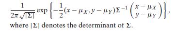
10. This exercise connects the form of bivariate normal PDF obtained in (4.6.3) through the principle of hierarchical modeling with its more common form given in(4.6.13). It also gives an alternative form of the PDF using matrix operations. For simplicity, ρ denotes ρX,Y.(a) Show that 1 − ρ2 =
9. An extensive study undertaken by the National Highway Traffic Safety Administration reported that 17% of children between the ages of five and six use no seat belt, 29% use a seat belt, and 54% use a child seat. In a sample of 15 children between five and six let N1,N2,N3 be the number of
8. Suppose that 60% of the supply of raw material kits used in a chemical reaction can be classified as recent, 30% as moderately aged, 8% as aged, and 2% unusable.Sixteen kits are randomly chosen to be used for 16 chemical reactions. Let N1,N2,N3,N4 denote the number of chemical reactions
7. The exponential regression model. The exponential regression model is common in reliability studies investigating how the expected life time of a product changes with some operational stress variable X. This model assumes that the life time, Y, has an exponential distribution whose parameter λ
6. Use the second mean plus error expression of the response variable given in (4.6.6) and Proposition 4.4-2 to derive the formula E(Y) = β0. (Hint. Recall that any(intrinsic) error variable has mean value zero.)
5. Consider the information given in Exercise 3. Suppose further that the marginal distribution of X is normal withμX = 24 and σ2X= 9.(a) Give the joint PDF of X,Y.(b) Use R commands to find P(X ≤ 25,Y ≤ 45).
4. Consider the information given in Exercise 3. Suppose further that the marginal mean and variance of X are E(X) = 24 and σ2X= 9, and the marginal variance of Y is σ2Y= 36.25.(a) Find the marginal mean of Y. (Hint. Use Proposition 4.6-1, or the Law of Total Expectation given in 4.3.15.)(b) Find
3. In the context of the normal simple linear regression model Y|X = x ∼ N(9.3 + 1.5x, 16), let Y1, Y2 be independent observations corresponding to X = 20 and X = 25, respectively.(a) Find the 95th percentile of Y1.(b) Find the probability that Y2 > Y1. (Hint. See Example 4.6-4.)
2. Consider the same setting as in Exercise 1, except now P is assumed here to have the uniform(0, 1) distribution.(a) Use the principle of hierarchical modeling to specify the joint density of fP,Y(p, y) of (P,Y) as the product of the conditional PMF of Y given P = p times the marginal PDF of

Showing 1900 - 2000 of 2867

First
13
14
15
16
17
18
19
20
21
22
23
24
25
26
27
Last

Step by Step Answers

Services

Sitemap
Fun
Definitions
Become Tutor
Used Textbooks
Study Help Categories
Recent Questions
Expert Questions
Campus Wear
Sell Your Books

Company Info

Security
Copyrights
Privacy Policy
Terms & Conditions
SolutionInn Fee
Scholarship
Online Quiz
Give Feedback, Get Rewards

Get In Touch

About Us
Contact Us
Career
Jobs
FAQ
Student Discount
Campus Ambassador

Secure Payment

Download Our App

© 2026 SolutionInn. All Rights Reserved