New Semester Started Get 50% OFF Study Help! --h --m --s Claim Now

Question Answers

Textbooks

Find textbooks, questions and answers

Oops, something went wrong!

Change your search query and then try again

Result Not Found

Books FREE
Study Help
Tutors
AI Study Planner NEW
Sell Books

Search
Sign In
Register

study help
business
bayesian statistics an introduction

Probability & Statistics For Engineers And Scientists With R 1st Edition Michael Akritas - Solutions

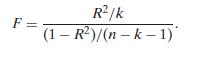
6. Show that the F statistic for the model utility test given in (12.3.17) can be expressed in terms of R2 as F= R/k (1 R2)/(n-k-1)
5. The data in EmployPostRecess.txt has the number of employees of a particular company during 11 postrecession quarters. Import the data into the R data frame pr and use x=pr$Quarter; xc=x-mean(x); y=pr$Population to set the centered predictor and the response variable in the R objects x and y,
4. The file HardwoodTensileStr.txt has data on hardwood concentration and tensile strength.5 Import the data into the R data frame hc and use x=hc$Concentration; x=xmean(x); y=hc$Strength to set the centered predictor and the response variable in the R objects x and y, respectively.(a) Use
3. The R data set state.x77, collected by the US Bureau of the Census in the 1970s, has the population, per capita income, illiteracy, life expectancy, murder rate, percent high school graduation, mean number of frost days(defined as days with minimum temperature below freezing in the capital or a
2. The R data set stackloss4 contains data from 21 days of operation of a plant whose processes include the oxidation of ammonia (NH3) to nitric acid (HNO3).The nitric-oxide wastes produced are absorbed in a countercurrent absorption tower. There are three predictor variables: Air.Flow represents
1. An article reports on a study of methyl tertiarybutyl ether (MTBE) in the vicinity of two gas stations, one urban and one roadside, equipped with stage I vapor recovery systems.3 The data set in GasStatPoll.txt contains the MTBE concentration measurements along with the covariates “Gas
For the data of Example 12.3-1, use R commands to fit the model that includes second order polynomial terms in latitude and longitude, as well as the latitudelongitude interaction, and to complete the following parts. (a) Construct 90% CIs for each of the six regression coefficients.(b) Construct a
For the temperature-latitude-longitude data set of Example 12.3-1, let X1 and X2 denote the centered latitude and longitude variables, and use R commands to complete the following parts.(a) Fit the model that includes second order polynomial terms in X1 and X2 and X1X2 (the X1X2 interaction term),
For each of models (1) and (3) mentioned in Example 12.3-1 for the temperaturelatitude-longitude data set, do the following.(a) Carry out the model utility test at level α = 0.01 and report the p-value.(b) Use diagnostic plots and formal tests to test the assumptions of homoscedasticity and
Consider the first 8 of the 56 data points of the temperature-latitude-longitude data set of Example 12.3-1.(a) Give the design matrices for models (1) and (2) specified in Example 12.3-1.(b) Write the normal equations for model (1) and obtain the least squares estimators.(c) Give the estimated
The data2 in Temp.Long.Lat.txt give the average (over the years 1931 to 1960) daily minimum January temperature in degrees Fahrenheit with the latitude and longitude of 56 US cities. Let Y, X1, X2 denote the temperature and the centered latitude and longitude variables, respectively.(a) Using R
6. The data set in WindSpeed.txt has 25 measurements of current output, produced by a wind mill, and wind speed(in miles per hour).1 Import the wind speed and output into the R objects x and y, respectively.(a) Construct the (x, y) and (1/x, y) scatterplots. Which scatterplot suggests a linear
5. The file BacteriaDeath.txt has simulated data on bacteria deaths over time. Import the time and bacteria counts into the R objects t and y, respectively.(a) Construct the (t, y) and (t, log(y)) scatterplots. Which scatterplot suggests a linear relationship?(b) Construct a predictive equation for
4. The data set Leinhardt in the R package car has data on per capita income and infant mortality rate from several countries. Use the R commands install.packages(”car”) to install the package, the command library(car) to make the package available to the current R session, and the command
3. A response variable is related to a predictor variable through the quadratic regression model μY|X(x) = −8.5− 3.2x + 0.7x2.(a) Give the rate of change of the regression function at x = 0, 2, and 3.(b) Express the model in terms of the centered variables as μY|X(x) = β0 + β1(x − μX) +
2. A response variable is related to two predictors through the multiple regression model with an interaction term Y = 3.6 + 2.7X1 + 0.9X2 + 1.5X1X2 + ε.(a) If E(X1) = 10, E(X2) = 18, and Cov(X1,X2) = 80, find the (marginal) expected value of Y. (Hint.Cov(X1,X2) = E(X1X2) − E(X1)E(X2).)(b)
1. A response variable is related to two predictors through the multiple linear regression model Y = 3.6 + 2.7X1 + 0.9X2 + ε.(a) Give μY|X1,X2 (12, 25) = E(Y|X1 = 12,X2 = 25).(b) If E(X1) = 10 and E(X2) = 18, find the (marginal)expected value of Y.(c) What is the expected change in Y when X1
11. Photomasks are used to generate various design patterns in the fabrication of liquid crystal displays (LCDs).A paper11 reports on a study aimed at optimizing process parameters for laser micro-engraving iron oxide coated glass. The effect of five process parameters was explored(letter
10. Answer the following questions.(a) Construct a 25−1 design, using the five-factor interaction as the generator effect, and give the set of(25 − 2)/2 = 15 aliased pairs.(b) Construct a 26−2 fractional factorial design using ABCE and BCDF as the generator effects. Give the third
9. Verify that the set of alias pairs in the 23−1 designare the same as those for its complimentary 23−1 design given in Table 11-4. (Hint. Write the contrast corresponding to each main effect column, as was done in (11.4.6), and find what it estimates, as was done in (11.4.7).) Factor-Level
8. Consider the 23−1 design shown in Table 11-4, and verify that β1 is confounded with (αγ )11 and γ1 is confounded with (αβ)11.
7. Arc welding is one of several fusion processes for joining metals. By intermixing the melted metal between two parts, a metallurgical bond is created resulting in desirable strength properties. A study investigated the effect on the strength of welded material (factor A at levels SS41 and SB35),
6. In the context of Exercise 5, the experiment accounted for the possible influence of the blocking factor “tool inserts” at two levels, with the eight runs allocated into four blocks in such a way that the interactions AB, AC, and their generalized interaction, which is BC, are confounded
5. A paper presents a study investigating the effects of feed rate (factor A at levels 50 and 30), spindle speed(factor B at levels 1500 and 2500), depth of cut (factor C at levels 0.06 and 0.08), and the operating chamber temperature on surface roughness.10 In the data shown in SurfRoughOptim.txt,
4. A 25 design will be run in eight blocks. Let the five factors be denoted by A, B, C, D, and E.(a) What is the total number of effects that must be confounded with the block effects?(b) Construct the set of confounded effects from the defining effects ABC, BCD, and CDE.(c) Use R commands to find
3. A 25 design will be run in four blocks. Let the five factors be denoted by A, B, C, D, and E.(a) Find the generalized interaction of the defining effects ABC and CDE.(b) Find the generalized interaction of the defining effects BCD and CDE.(c) For each of the two cases above, use R commands to
2. Verify the following:(a) Use the first of the two commands given in (11.4.3)to verify that the block effect is confounded only with the main effect of factor A.(b) Use the second of the two commands given in (11.4.3)to verify that the block effect is confounded only with the BC interaction
1. Verify that the treatment allocation to blocks described in Figure 11-6 confounds only the three-factor interactions with the block effect. (Hint. The contrasts estimating the different effects are given in Example 11.3-1.)
The data in Ffd.2.5-2.txt are from an experiment using a 25−2 design with treatment combinations given in Example 11.4-3.(a) Compute the sums of squares for each class of aliased effects using (11.4.9).(b) Assuming that one class of aliased effects is zero (or negligible), test for the
Due to time considerations, an accelerated life testing experiment is conducted in two labs. There are two levels for each of the three factors involved and the experimental runs are allocated in the two labs so that the lab effect is confounded only with the three-factor interaction effect; see
6. Let μ, αi, (αβ)ij, (αβγ )ijk, etc., be the terms in the decomposition (11.3.1), and letμk = μ··k, αk i = μi·k − μk,βk j = μ·jk − μk, (αβ)k ij = μijk − μk − αk i − βk j , be the terms in the decomposition (11.3.4) when the level of factor C is held fixed at k.
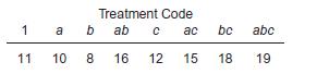
5. Assume the 23 design of Example 11.3-1 has only one replication, that is, n = 1, with the observations as given in Table 11-1. Use hand calculations to complete the following.(a) The estimated main and interaction effects computed in Example 11.3-1 remain the same. True or false? If you answer
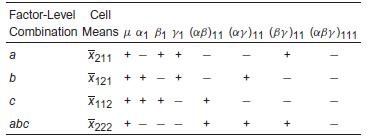
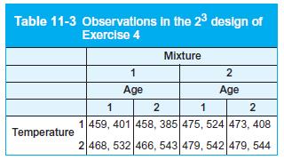
4. The data shown in Table 11-3 are from an experiment investigating the compressive strength of two different mixtures at two temperatures and two aging periods.(a) Compute a table of signs for estimating the main and interaction effects, similar to Table 11-2. (Include the first column of
3. Line yield and defect density are very important variables in the semiconductor industry as they are directly correlated with production cost and quality. A small pilot study considered the effect of three factors, “PMOS transistor threshold voltage,” “polysilicon sheet resistance,”and
2. In a study of the effectiveness of three types of home insulation methods in cold weather, an experiment considered the energy consumption, in kilowatt hours (kWh) per 1000 square feet, at two outside temperature levels (15o–20oF and 25o–30oF), using two different thermostat settings
1. A number of studies have considered the effectiveness of membrane filtration in removing or rejecting organic micropollutants. Membranes act as nano-engineered sieves and thus the rejection rate depends on the molecular weight of the pollutant or solute. In addition, the rejection rate depends
A paper reports on a study sponsored by CIFOR (Center for International Forestry Research) to evaluate the effectiveness of monitoring methods related to water and soil management.6 Part of the study considered soil runoff data from two catchment areas (areas number 37 and 92) using runoff plots
Hand calculations in a 23 design. Surface roughness is of interest in many manufacturing processes. A paper5 considers the effect of several factors including tip radius(TR), surface autocorrelation length (SAL), and height distribution (HD) on surface roughness, on the nanometer scale, by the
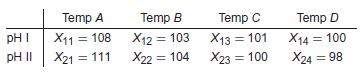
12. A soil scientist is considering the effect of soil pH level (factor A) on the breakdown of a pesticide residue.Two pH levels are considered in the study. Because pesticide residue breakdown is also affected by soil temperature(factor B), four different temperatures are included in the study.
11. Data from an article investigating the effect of auxincytokinin interaction on the organogenesis of haploid geranium callus can be found in AuxinKinetinWeight.txt.4 Read the data into the data frame Ac, and use attach(Ac);A=as.factor(Auxin); B=as.factor(Kinetin); y=Weight to copy the response
10. Consider the cellphone radiation data of Exercise 2, but use one observation per cell. (This serves to highlight the additional power gained by using several observations per factor-level combination.) Having imported the data into the data frame df, use y = df $y[1 : 15], S = df $S[1:15], C =
9. The data file InsectTrap.txt contains the average number of insects trapped for three kinds of traps used in five periods.3 Read the data into the data frame df, set y=df$catch; A=as.factor(df$period); B=as.factor(df$trap), and use R commands to complete the following.(a) Construct the ANOVA F
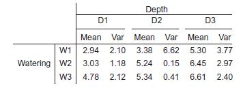
8. It is known that the life span of a particular type of root system is influenced by the amount of watering it receives and its depth. An experiment is designed to study the effect of three watering regimens (“W1,” “W2,” “W3”), and their possible interaction with the depth factor. The
7. When an additive model is considered for a balanced design, the decomposition of the total sum of squares in(11.2.10) reduces to SST = SSA+SSB+SSE, where SST and its degrees of freedom are still given by (11.2.9), and SSA, SSB, and their degrees of freedom are still given by(11.2.11) and
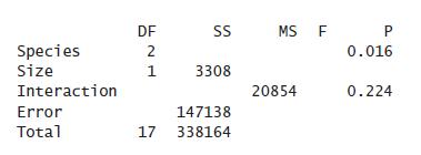
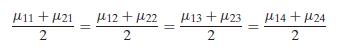
6. A large research project studied the physical properties of wood materials constructed by bonding together small flakes of wood. Three different species of trees(aspen, birch, and maple) were used, and the flakes were made in two different sizes (0.015 inches by 2 inches and 0.025 inches by 2
5. The data file AdLocNews.txt contains the number of inquiries regarding ads placed in a local newspaper. The ads are categorized according to the day of the week and section of the newspaper in which they appeared. Use R commands to complete the following:(a) Construct plots to help assess the
4. The data file AdhesHumTemp.txt contains simulated data from a study conducted to investigate the effect of temperature and humidity on the force required to separate an adhesive product from a certain material. Two temperature settings (20◦, 30◦) and four humidity settings(20%, 40%, 60%,
3. The data file Alertness.txt contains data from a study on the effect on alertness of two doses of a medication on male and female subjects. This is a 2 × 2 design with four replications. The question of interest is whether changing the dose changes the average alertness of male and female
2. A cellphone’s SAR (Specific Absorption Rate) is a measure of the amount of radio frequency (RF) energy absorbed by the body when using the handset. For a phone to receive FCC certification, its maximum SAR level must be 1.6 watts per kilogram (W/kg); the level is the same in Canada, while in
1. An experiment studying the effect of growth hormone and sex steroid on the change in body mass fat in men resulted in the data shown in GroHormSexSter.txt (P, p for placebo, and T, t for treatment).2 This is an unbalanced design with sample sizes n11 = 17, n12 = 21, n21 = 17, n22 = 19, where
Use R commands to generate data from an additive, and also from a non-additive, 3 × 3 design with one observation per cell and non-zeromain effects.(a) Apply Tukey’s one degree of freedom test for interaction to both data sets, stating whether or not the additivity assumption is tenable.(b)
Check whether the data of Examples 11.2-1 and 11.2-2 satisfy the homoscedasticity and normality assumptions.
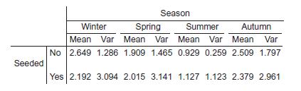
The data file CloudSeed2w.txt contains the rainfall measurements of the previous example. Use R commands to construct the ANOVA table and to perform Tukey’s 95% simultaneous CIs and multiple comparisons for determining the pairs of seasons that are significantly different at experiment-wise error
Data were collected1 on the amount of rainfall, in inches, in select target areas of Tasmania with and without cloud seeding during the different seasons. The sample means and sample variances of the n = 8 measurements from each factor-level combination are given in the table below.Carry out the
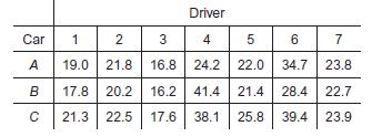
7. A study was conducted to see whether three cars, A, B, and C, took the same time to parallel park. A random sample of seven drivers was obtained and the time required for each of them to parallel park each of the three cars was measured. The results are listed in the table below.Is there
6. The data file FabricStrengRbd.txt contains the fabric strength data of Exercise 5. Import the data into the R object fs, and use the R commands ranks=rank(fs$streng);anova(aov(ranks∼ fs$chemical+fs$fabric))to construct the ANOVA table on the ranks.(a) Report the p-value for testing the null
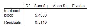
5. An experiment was performed to determine the effect of four different chemicals on the strength of a fabric.Five fabric samples were selected and each chemical was tested once in random order on each fabric sample. The total sum of squares for this data is SST = 8.4455. Some additional summary
4. In the context of Exercise 3, use R commands to construct Tukey’s 99% simultaneous CIs, including the plot that visually displays them, and perform multiple comparisons at experiment-wise level 0.01 to determine which pairs of designs differ significantly in terms of the pilot’s response
3. A commercial airline is considering four different designs of the control panel for the new generation of airplanes.To see if the designs have an effect on the pilot’s response time to emergency displays, emergency conditions were simulated and the response times, in seconds, of 8 pilots were
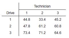
2. A service center for electronic equipment is interested in investigating possible differences in service times of the three types disk drives that it regularly services. Each of the three technicians currently employed was randomly assigned to one repair of each type of drive and the repair
1. The data for the rate of combustion in humid air flow study of Exercise 5 in Section 10.2 can be found in CombustRate.txt. In the context of that exercise, an engineer with statistical training observes that there is a certain pattern in the data and inquires about other experimental conditions.
In the context of the wine tasting data of Example 10.4-3, apply Tukey’s method to construct 95% simultaneous CIs and multiple comparisons to identify which of the/42 0= 6 pairs of wines are significantly different at experiment-wise level of significance α = 0.05.
In the context of the wine tasting data of Example 10.4-3, apply the following Bonferroni multiple comparisons procedures to identify which of the/42 0= 6 pairs of wines are significantly different at experiment-wise level of significance α = 0.05.(a) Construct 95% Bonferroni simultaneous CIs, and
For the wine tasting data set of Example 10.4-3, the summary statistics on the within-block ranks rij are r1· = 3.11, r2· = 3.14, r3· = 1.92, r4· = 1.83, and r·· = 2.5. Moreover, the sample variance of these ranks is 1.248. With the information given, calculate Friedman’s test statistic and
For the wine tasting data set of Example 10.4-3, the summary statistics on the ranks are R1· = 90.93, R2· = 94.89, R3· = 52.97, R4· = 51.21, and R·· = 72.50. Moreover, it is given that the rank sum of squares due to the visitors (blocks) is SSBR = 41,843 and the rank total sum of squares is
A randomsample of 36 Napa Valley visitors tested and rated four wine varieties on a scale of 1–10. For impartiality purposes, thewineswere identified only by numbers 1–4. The order in which each of the four wines were presented to each visitor was randomized. The average rating for each wine,
8. For the data in Exercise 12 in Section 10.2, use the Bonferroni multiple comparisons method to identify the groups whose population proportions differ significantly at experiment-wise level of significance α = 0.05.
7. For the data in Exercise 10 in Section 10.2, construct Bonrerroni 95% simultaneous CIs for all pairwise differences of proportions, and use them to identify the pairs of proportions that differ at experiment-wise level of significance 0.05.
6. Consider the data in Exercise 5.(a) Conduct the Kruskal-Wallis test at level α = 0.05 and state what assumptions, if any, are needed for its validity.(b) Use the Bonferroni multiple comparisons method with the rank-sum test to identify the groups whose population means differ significantly at
5. Records from an honors statistics class, Experimental Design for Engineers, indicated that each professor had adopted one of three different teaching methods: (A) use of a textbook as the main source of teaching material,(B) use of a textbook combined with computer activities, and (C) use of
4. Consider the setting and data of Exercise 6 in Section 10.2.(a) Use R commands or hand calculations to compute Tukey’s 95% simultaneous CIs, and perform Tukey’s multiple comparisons at experiment-wise level of significanceα = 0.05. (Hint. You may use the summary statistics given in Exercise
3. A study conducted at Delphi Energy & Engine Management Systems considered the effect of blow-off pressure during the manufacture of spark plugs on the spark plug resistance. The resistance measurements of 150 spark plugs manufactured at each of three different blow-off pressures (10, 12, and 15
2. Consider the data in Exercise 8 in Section 10.2 on fixed-platen compression strengths of three types of corrugated fiberboard containers.(a) One of the assumptions needed for the validity of the ANOVA F test is homoscedasticity, or equal variances.Since only summary statistics are given, the
1. An article reports on a study using high temperature strain gages to measure the total strain amplitude of three different types of cast iron [spheroidal graphite (S), compacted graphite (C), and gray (G)] for use in disc brakes.4 Nine measurements from each type were taken and the results
Consider the setting of Example 10.2-4, where three types of fabric are tested for their flammability, and use Tukey’s multiple comparisons method on the ranks to identify which materials differ in terms of flammability at experiment-wise level of significance α = 0.1.
Iron concentration measurements from four ore formations are given in FeData.txt.Use Bonferroni multiple comparisons, based on rank-sum tests, to determine which pairs of ore formations differ, at experiment-wise level of significance α = 0.05, in terms of iron concentration.
In the context of Example 10.2-5, use multiple comparisons based on Bonferroni simultaneous CIs to determine which pairs of panel designs differ, at experimentwise level of significance α = 0.05, in terms of their effect on the pilot’s reaction time.
12. Wind-born debris (from roofs, passing trucks, insects, or birds) can wreak havoc on architectural glass in the upper stories of a building. A paper reports the results of an experiment where 10 configurations of glass were subjected to a 2-gram steel ball projectile traveling under 5 impact
11. A certain brand of tractor is assembled in five different locations. To see if the proportion of tractors that require warranty repair work is the same for all locations, a random sample of 50 tractors from each location is selected and followed up for the duration of the warranty period. The
10. The flame resistance of three materials used in children’s pajamas was tested by subjecting specimens of the materials to high temperatures. Out of 111 specimens of material A, 37 ignited.Out of 85 specimens ofmaterial B, 28 ignited. Out of 100 specimens of material C, 21 ignited.Test the
9. An article reports on a study where fatigue tests were performed by subjecting the threaded connection of large diameter pipes to constant amplitude stress of either L1= 10 ksi, L2 = 12.5 ksi, L3 = 15 ksi, L4 = 18 ksi, or L5 = 22 ksi.2 The measured fatigue lives, in number of cycles to failure
8. Compression testing of shipping containers aims at determining if the container will survive the compression loads expected during distribution. Two common types of compression testers are fixed platen and floating platen. The two methods were considered in a study, using different types of
7. Consider the setting and data of Exercise 6.(a) Use hand calculations to conduct the Kruskal-Wallis test at level α = 0.05, stating any assumptions needed for its validity. (Hint. This data set has ties. You may use attach(pc); ranks=rank(values);vranks=var(ranks); rms= by(ranks, temp, mean) to
6. Porous carbon materials are used commercially in several industrial applications, including gas separation, membrane separation, and fuel cell applications. For the purpose of gas separation, the pore size is important.To compare the mean pore size of carbon made at temperatures (in ◦C) of
5. As part of a study on the rate of combustion of artificial graphite in humid air flow, researchers conducted an experiment to investigate oxygen diffusivity through a water vapor mixture. An experiment was conducted with mole fraction of water at levels MF1 = 0.002, MF2 = 0.02, and MF3 = 0.08.
4. Consider the setting and data of Exercise 3.(a) Use hand calculations to conduct the Kruskal-Wallis test at level α = 0.05, stating any assumptions needed for its validity. (Hint. There are no ties in this data set. You may use attach(sl); ranks=rank(values);rms=by(ranks, ind, mean) to compute
3. Four different concentrations of ethanol are compared at level α = 0.05 for their effect on sleep time. Each concentration was given to a sample of 5 rats and the REM (rapid eye movement) sleep time for each rat was recorded (SleepRem.txt). Do the four concentrations differ in terms of their
2. In the context of Example 10.2-4, where three types of fabric are tested for their flammability, materials 1 and 3 have been in use for some time and are known to possess similar flammability properties. Material 2 has been recently proposed as an alternative. Of primary interest in the study is
1. In a study aimed at comparing the average tread lives of four types of truck tires, 28 trucks were randomly divided into four groups of seven trucks.Each group of seven trucks was equipped with tires from one of the four types. The data in TireLife1 Way.txt consist of the average tread lives of
A commercial airline is considering four different designs of the control panel for the new generation of airplanes. To see if the designs have an effect on the pilot’s response time to emergency displays, emergency conditions were simulated and the response times of pilots were recorded. The
Organizations such as the American Society for Testing Materials are interested in the flammability properties of clothing textiles. A particular study performed a standard flammability test on six pieces from each of three types of fabric used in children’s clothing. The response variable is the
In the context of the water quality measurements of Example 10.2-2, test the validity of the assumptions of equal variances and normality.
A quantification of coastal water quality converts measurements on several pollutants to a water quality index with values from 1 to 10. An investigation into the after-clean-up water quality of a lake focuses on five areas encompassing the two beaches on the eastern shore and the three beaches on
To compare three different mixtures of methacrylic acid and ethyl acrylate for stain/soil release effectiveness, 5 cotton fabric specimens are treated with each mixture and tested. The data are given in FabricSoiling.txt. Do the three mixtures differ in the stain/soil release effectiveness? Test at
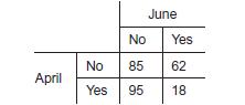
6. To assess a possible change in voter attitude toward gun control legislation between April and June, a random sample of n = 260 was interviewed in April and in June.The resulting responses are summarized in the following table:Is there evidence that there was a change in voter attitude?Test at
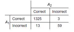
5. During the evaluation of two speech recognition algorithms, A1 and A2, each is presented with the same sequence, u1, . . . , un, of labeled utterances for recognition.The {ui} are assumed to be a random sample from some population of utterances. Each algorithm makes a decision about the label of
4. Two brands of motorcycle tires are to be compared for durability. Eight motorcycles are selected at random and one tire from each brand is randomly assigned (front or back) on each motorcycle. The motorcycles are then run until the tires wear out. The data, in km, are given in
3. The percent of soil passing through a sieve is one of several soil properties studied by organizations such as the National Highway Institute. A particular experiement considered the percent of soil passing through a 3/8-inch sieve for soil taken from two separate locations. It is known that the
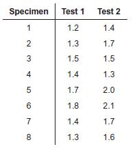
2. Two different analytical tests can be used to determine the impurity levels in steel alloys. The first test is known to perform very well but the second is cheaper. A specialty steel manufacturer will adopt the second method unless there is evidence that it gives significantly different results
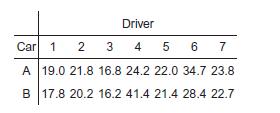
1. A study was conducted to see whether two types of cars, A and B, took the same time to parallel park. Seven drivers were randomly obtained and the time required for each of them to parallel park each of the 2 cars was measured. The results are listed in the following table.Is there evidence that

Showing 1700 - 1800 of 2867

First
11
12
13
14
15
16
17
18
19
20
21
22
23
24
25
Last

Step by Step Answers

Services

Sitemap
Fun
Definitions
Become Tutor
Used Textbooks
Study Help Categories
Recent Questions
Expert Questions
Campus Wear
Sell Your Books

Company Info

Security
Copyrights
Privacy Policy
Terms & Conditions
SolutionInn Fee
Scholarship
Online Quiz
Give Feedback, Get Rewards

Get In Touch

About Us
Contact Us
Career
Jobs
FAQ
Student Discount
Campus Ambassador

Secure Payment

Download Our App

© 2026 SolutionInn. All Rights Reserved