New Semester
Started
Get
50% OFF
Study Help!
--h --m --s
Claim Now
Question Answers
Textbooks
Find textbooks, questions and answers
Oops, something went wrong!
Change your search query and then try again
S
Books
FREE
Study Help
Expert Questions
Accounting
General Management
Mathematics
Finance
Organizational Behaviour
Law
Physics
Operating System
Management Leadership
Sociology
Programming
Marketing
Database
Computer Network
Economics
Textbooks Solutions
Accounting
Managerial Accounting
Management Leadership
Cost Accounting
Statistics
Business Law
Corporate Finance
Finance
Economics
Auditing
Tutors
Online Tutors
Find a Tutor
Hire a Tutor
Become a Tutor
AI Tutor
AI Study Planner
NEW
Sell Books
Search
Search
Sign In
Register
study help
business
bayesian statistics an introduction
Bayesian Statistics An Introduction 4th Edition Peter M. Lee - Solutions
Suppose that the standard test statistic z = (X̅- θ0)/√(ϕ/n) takes the value z = 2.5 and that the sample size is n = 100. How close to θ0 does a value of θhave to be for the value of the normal likelihood function at X̅ to be within 10% of its value at θ = θ0?
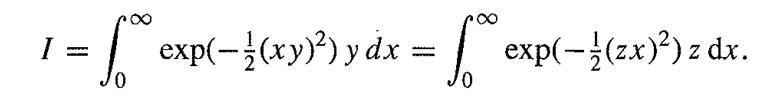
Show that the Bayes factor for a test of a point null hypothesis for the normal distribution (where the prior under the alternative hypothesis is also normal) can be expanded in a power series in λ = ϕψ as B = λ exp(-2²){1 + ½ λ(z² + 1) + · · ·}.
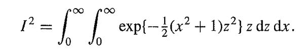
At the beginning of Section 4.5, we saw that under the alternative hypothesis that θ ~ N(θ,ψ) the predictive density for X̅ was N(θ0, ψ + ϕ), so thatShow that a maximum of this density considered as a function of ψ occurs when ψ = (z2 - 1)ϕ, which gives a possible value for ψ if z ≥
In the situation discussed in Section 4.5, for a given P-value (so equivalently for a given z) and assuming that ϕ = ψ, at what value of n is the posterior probability of the null hypothesis a minimum.
Mendel (1865) reported finding 1850 angular wrinkled seeds to 5474 round or roundish in an experiment in which his theory predicted a ratio of 1: 3. Use the method employed for Weldon's dice data in Section 4.5 to test whether his theory is confirmed by the data. [However, Fisher (1936) cast some
A window is broken in forcing entry to a house. The refractive index of a piece of glass found at the scene of the crime is x, which is supposed N(θ1,ϕ). The refractive index of a piece of glass found on a suspect is y, which is supposed N(θ2,ϕ). In the process of establishing the guilt or
Lindley (1957) originally discussed his paradox under slightly different assumptions from those made in this book. Follow through the reasoning used in Section 4.5 with P1 (θ) representing a uniform distribution on the interval (θ0 - ½ τ, θ0 + ½τ) to find the corresponding Bayes factor
Express in your own words the arguments given by Jeffreys (1961, Section 5.2) in favour of a Cauchy distributionin the problem discussed in the previous question.Previous questionLindley (1957) originally discussed his paradox under slightly different assumptions from those made in this book.
Suppose that x has a binomial distribution B(n, θ) of index n and parameter 0, and that it is desired to test H0 : θ = θ0 against the alternative hypothesis H1: θ ≠ θ0:(a) Find lower bounds on the posterior probability of H0 and on the Bayes factor for H0 versus H1, bounds which are valid
Twelve observations from a normal distribution of mean θ and variance ϕ are available, of which the sample mean is 1.2 and the sample variance is 1.1. Compare the Bayes factors in favour of the null hypothesis that 0 = θ0; assuming that (a) ϕ is unknown and (b) It is known that ϕ = 1.
Suppose that in testing a point null hypothesis you find a value of the usual Student's statistic of 2.4 on 8 degrees of freedom. Would the methodology of Section 4.6 require you to think again'?
Which entries in the table in Section 4.5 on 'Point null hypotheses for the normal distribution' would, according to the methodology of Section 4.6, cause you to 'think again'?Table in Section 4.5 P-value z\n 1 (2-tailed) 0.1 0.05 0.01 0.001 5 10 20 50 100 1000 1.645 0.418 0.442 0.492 0.558 0.655
Laplace claimed that the probability that an event which has occurred n times, and has not hitherto failed, will occur again is (n + 1)/(n + 2) [see Laplace (1774)], which is sometimes known as Laplace's rule of succession. Suggest grounds for this assertion.
Find a suitable interval of 90% posterior probability to quote in a case when your posterior distribution for an unknown parameter π is Be(20, 12), and compare this interval with similar intervals for the cases of Be(20.5, 12.5) and Be(21, 13) posteriors. Comment on the relevance of the results
Suppose that your prior beliefs about the probability π of success in Bernoulli trials have mean 1/3 and variance 1/32. Give a 95% posterior HDR for π given that you have observed 8 successes in 20 trials.
Suppose that you have a prior distribution for the probability π of success in a certain kind of gambling game which has mean 0.4, and that you regard your prior information as equivalent to 12 trials. You then play the game 25 times and win 12 times. What is your posterior distribution for π ?
Suppose that you are interested in the proportion of females in a certain organization and that as a first step in your investigation you intend to find out the sex of the first 11 members on the membership list. Before doing so, you have prior beliefs which you regard as equivalent to 25% of this
Show that if g(x) = sinh-1 √(x) thenDeduce that if x ~ NB(n,π) has a negative binomial distribution of index n and parameter π and z = g(x) then Ez ≅ sinh-1 √(x) and Vz ≅ 1/4n. What does this suggest as a reference prior for π ? g'(x) = {n¯¹[(x/n){1+(x/n)}]¯½.
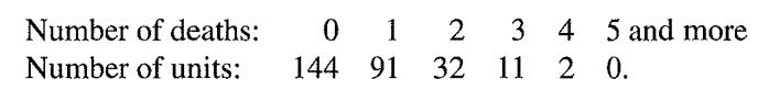
The following data were collected by von Bortkiewicz (1898) on the number of men killed by horses in certain Prussian army corps in twenty years, the unit being one army corps for one year:Give an interval in which the mean number λ of such deaths in a particular army corps in a particular year
Recalculate the answer to the previous question assuming that you had a prior distribution for λ of mean 0.66 and standard deviation 0.115.Previous questionThe following data were collected by von Bortkiewicz (1898) on the number of men killed by horses in certain Prussian army corps in twenty
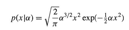
Find the Jeffreys prior for the parameter a of the Maxwell distribution and find a transformation of this parameter in which the corresponding prior is uniform. p(x|a) = 2 √/²=7a²³/²x² exp(-1αx²) X 2
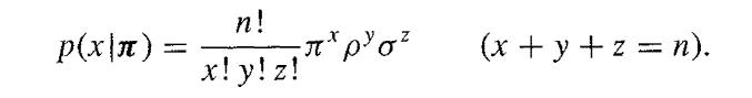
Use the two-dimensional version of Jeffreys' rule to determine a prior for the trinomial distribution(cf. Exercise 15 on Chapter 2).Exercise 15Suppose that the vector x = (x, y, z) has a trinomial distribution depending on the index n and the parameter π = (π , p, σ), where π + p + σ = 1,
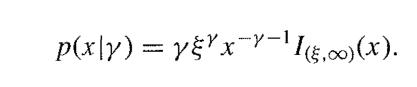
Suppose that x has a pareto distributionPa(ξ, y ), where ξ is known but y is unknown, that isUse Jeffreys' rule to find a suitable reference prior for y. p(x|y) = yx-¹(5,0)(x).
Consider a uniform distribution on the interval (a, β), where the values of a and β are unknown, and suppose that the joint distribution of a and β is a bilateral bivariate Pareto distribution with y = 2. How large a random sample must be taken from the uniform distribution in order that the
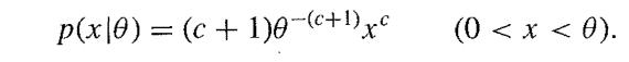
Suppose that observations x1, x2, ..., Xn are available from a densityExplain how you would make inferences about the parameter θ using a conjugate prior. p(x|0) = (c + 1)0−(c+¹) xc (0 < x < 0).
What could you conclude if you observed two tramcars numbered, say, 71 and 100?
We sometimes investigate distributions on a circle. Find a Haar prior for a location parameter on the circle (such as µ, in the case of von Mises' distribution).
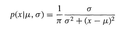
Suppose that the prior distribution p(µ,σ) for the parameters µ, and σ of a Cauchy distributionis uniform in µ and σ, and that two observations x1 = 2 and x2 = 6 are available from this distribution. Calculate the value of the posterior density p(µ, σlx) (ignoring the factor 1/π2) to two
Show that if the log-likelihood L(θ I x) is a concave function of θ for each scalar x (that is, L"(θ l x) ≤ ( 0 for all θ), then the likelihood function L(θ l x) fore given an n-sample x = (x1, x2, ... , xn) has a unique maximum. Prove that this is the case if the observations xi come from a
Show that if an experiment consists of two observations, then the total information it provides is the information provided by one observation plus the mean amount provided by the second given the first.
Find the entropy H{p(θ)} of a (negative) exponential distribution with density p(θ) β-1 exp(-θ/β).
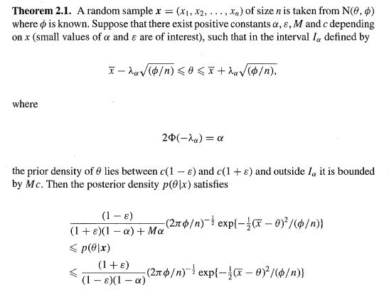
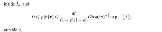
Prove the theorem quoted without proof in Section 2.4. Theorem 2.1. A random sample x = (x₁,x2,...,xn) of size n is taken from N(0, 0) where is known. Suppose that there exist positive constants a, e, M and c depending on x (small values of a and are of interest), such that in the interval la
Suppose that k ~ B(n, π). Find the standardized likelihood as a function of π for given k. Which of the distributions listed in Appendix A does this represent?Appendix A.Some facts are given about various common statistical distributions. In the case of continuous distributions, the (probability)
Suppose we are given the 12 observations from a normal distribution: and we are told that the variance ϕ = 1. Find a 90% HDR for the posterior distribution of the mean assuming the usual reference prior. 15.644, 16.437, 17.287, 14.448, 15.308, 15.169, 18.123, 17.635, 17.259, 16.311, 15.390,
With the same data as in the previous question, what is the predictive distribution for a possible future observation x?Previous questionSuppose we are given the 12 observations from a normal distribution: and we are told that the variance ϕ = 1. Find a 90% HDR for the posterior distribution of
A random sample of size n is to be taken from an N(θ,ϕ) distribution where ϕ is known. How large must n be to reduce the posterior variance of ϕ to the fraction ϕ/k of its original value (where k > 1)?
Your prior beliefs about a quantity θ are such thatA random sample of size 25 is taken from an N(θ, 1) distribution and the mean of the observations is observed to be 0.33. Find a 95% HDR for θ. p(0) = 1 (0 > 0) 0 (0 < 0).
Suppose that you have prior beliefs about an unknown quantity θ which can be approximated by an N(λ,ϕ) distribution, while my beliefs can be approximated by an N(μ,ψ) distribution. Suppose further that the reasons that have led us to these conclusions do not overlap with one another. What
Under what circumstances can a likelihood arising from a distribution in the exponential family be expressed in data translated form?
Suppose that you are interested in investigating how variable the performance of schoolchildren on a new mathematics test, and that you begin by trying this test out on children in 12 similar schools. It turns out that the average standard deviation is about 10 marks. You then want to try the test
The following are the dried weights of a number of plants (in g) from a batch of seeds:Give 90% HDRs for the mean and variance of the population from which they come. 4.17, 5.58, 5.18, 6.11, 4.50, 4.61, 5.17, 4.53, 5.33, 5.14.
Find a sufficient statistic for μ, given an n-sample x = (x1, x2 ,. . . , xn) from the exponential distributionwhere the parameter μ, can take any value in p(x|u) = μ΄' exp(-x/μ) (0 < x < )
Find a (two-dimensional) sufficient statistic for (a, β) given an n-sample x = (x1, x2,...,xn) from the two-parameter gamma distributionwhere the parameters a and β can take any values in p(x|a, B) = {pºr(a)}-xa-¹ exp(-x/B) (0 < x < ∞0)
Find a family of conjugate priors for the likelihood 1(β|x) = p(x|a,β), where p(x |a, β) is as in the previous question, but a is known.Previous questionFind a (two-dimensional) sufficient statistic for (a, β) given an n-sample x = (x1, x2,...,xn) from the two-parameter gamma distributionwhere
Show that the tangent of a random angle (i.e. one which is uniformly distributed on [0, 2π)) has a Cauchy distribution C(0,1).
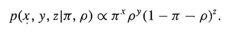
Suppose that the vector x = (x, y, z) has a trinomial distribution depending on the index n and the parameter π = (π , p, σ), where π + p + σ = 1, that isShow that this distribution is in the two-parameter exponential family. p(x|π) n! x!y!z! -π*p³σ² (x+y+z= n).
Suppose that the results of a certain test are known, on the basis of general theory, to be normally distributed about the same mean μ with the same variance ϕ, neither of which is known. Suppose further that your prior beliefs about (μ,ϕ) can be represented by a normal/chi-squared distribution
Suppose that your prior for θ is a 2/3 : 1/3 mixture of N(0, 1) and N(1, 1) and that a single observation x ~ N(θ, 1) turns out to equal 2. What is your posterior probability that θ > 1?
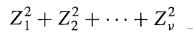
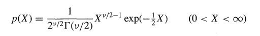
A random variable X is said to have a chi-squared distribution on v degrees of freedom if it has the same distribution as whcre Z1, Z2 , ... , Zv are independent standard normal variates. Use the facts that EZi = 0, EZ2i = 1 and EZ4i = 3 to find the mean and variance of X. Confirm these values
A card came is played with 52 cards divided equally between four players, North, South, East and West, all arrangements being equally likely. Thirteen of the cards are referred to as trumps. If you know that North and South have ten trumps between them, what is the probability that all three
(a) Under what circumstances is an event A independent of itself? (b) By considering events concerned with independent tosses of a r ~ d die and a blue die, or otherwise. give examples of events A, B and C which are not independent, but nevertheless are such that every pair of them is
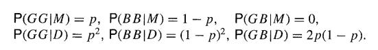
Whether certain mice are black or brown depends on a pair of genes, each of which is either B or b. If both members of the pair are alike, the mouse is said to be homozygous, and if they are different it is said to be heterozygous. The mouse is brown only it it is homozygous bb. The offspring of a
The example on Bayes' Theorem in Section 1.2 concerning the biology of twins was based on the assumption that births of boys arid girls occur equally frequently, and yet it has been known for a very long time that fewer girls are born than boys ( cf. Arbuthnot, 1710). Suppose that the probability
Suppose a red and a blue die are tossed. Let x be the sum of the number showing on the red die and twice the number showing on the blue die. Find the density function and the distribution function of x.
Suppose that k ~ B(n,π) where n is large and π is small but nπ = λ has an intermediate value. Use the exponential limit ( 1 + x )n → ex to show that P(k = 0) ≌ e-λ and P(k = I) ≌ λe-λ . Extend this result to show that k is such that that is, k is approximately distributed as a
Suppose that m and n have independent Poisson distributions of means λ and µ, respectively (see question 6) and that k = m + n. (b) Generalize by showing that k has a Poisson distribution of mean λ + µ. (c) Show that conditional on k, the distribution of m is binomial of index k and parameter
Modify the formula for the density of a one-to-one function g(x) of a random variable x to find an expression for the density of x2 in terms of that of x, in both the continuous and discrete case. Hence, show that the square of a standard normal density has a chi-squared density on one degree of
Suppose that x1, x2 , ... , Xn are independently and all have the same continuous distribution, with density f(x) and distribution function F(x). Find the distribution functions ofin terms of F(x), and so find expressions for the density functions of M and m. M = max{x₁, x2,...,xn) and m =
Suppose that u and v are independently uniformly distributed on the interval [0, 1], so that the divide the interval into three sub-intervals. Find the joint density function of the lengths of the first two sub-intervals.
Show that two continuous random variables x and y are independent (i.e. p(x, y) = p(x )p(y) for all x and y) if and only if their joint distribution function F(x, y) satisfies F(x, y) = F(x) F(y) for all x and y. Prove that the same thing is true for discrete random variables. [This is an example
Suppose that the random variable x has a negative binomial distribution NB(n, π) of index n and parameter π , so thatFind the mean and variance of x and check that your answer agrees with that given in Appendix A.Appendix A.Some facts are given about various common statistical distributions. In
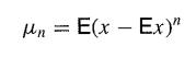
The skewness of a random variable x is defined as y1 = µ3/(µ,2) 3/2 where
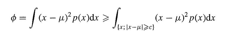
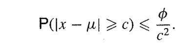
Suppose that a continuous random variable X has meanµ, and variance ϕ. By writing and using a lower bound for the integrand in the latter integral, prove that Show that the result also holds for discrete random variables. [This result is known as Cebysev's Inequality (the name is spelt in many
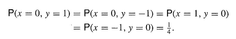
Suppose that x and y are such that Show that x and y are uncorrelated but that they are not independent. P(x = 0, y = 1) = P(x = 0, y = − 1) = P(x = 1, y = 0) = P(x = -1, y = 0) = 1.
Let x and y have a bivariate normal distribution and suppose that x and y both have mean 0 and variance 1, so that their marginal distributions arc standard normal and their joint density is Show that if the correlation coefficient between x and y is p, then that between x2 and y2 is p2. p(x, y) =
Suppose that x has a Poisson distribution (see question 6) P(λ) of mean λ and that, for given x, y has a binomial distribution B(x,π) of index x and parameter π.(a) Show that the unconditional distribution of y is Poisson of mean (b) Verify that the formula derived in Section 1.5 holds in
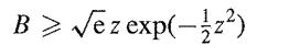
Define and show (by setting z = xy and then substituting z for y) thatDeduce that By substituting (I + x2)z2 = 2t, so that z dz = dt /(1 + x2) show that I = √π/2, so that the density of the standard normal distribution as defined in Section 1.3 does integrate to unity and so is indeed a
Showing 2800 - 2900
of 2867
First
15
16
17
18
19
20
21
22
23
24
25
26
27
28
29
Step by Step Answers
![P(x) = {2(y +)} exp[-(x 00)/(y + p)].](https://dsd5zvtm8ll6.cloudfront.net/images/question_images/1700/9/3/7/7836562403754b9b1700937776800.jpg)

![g'(x) = {n[(x){1+(x)}].](https://dsd5zvtm8ll6.cloudfront.net/images/question_images/1700/9/2/9/21765621ec11943c1700929210947.jpg)


![M = max(x, x2, ..., Xn] and m= min{x, x2, ..., Xn}](https://dsd5zvtm8ll6.cloudfront.net/images/question_images/1700/9/1/1/9946561db7a612911700911987886.jpg)
![-1 p(x, y) = {2 (1- p)] ' exp{- (x 2pxy + y)/(1 p)}. .](https://dsd5zvtm8ll6.cloudfront.net/images/question_images/1700/9/2/3/112656206e8440431700923107095.jpg)
![J = ] = exp(-1/z) dz](https://dsd5zvtm8ll6.cloudfront.net/images/question_images/1700/9/2/3/634656208f23d0111700923628090.jpg)