New Semester Started Get 50% OFF Study Help! --h --m --s Claim Now

Question Answers

Textbooks

Find textbooks, questions and answers

Oops, something went wrong!

Change your search query and then try again

Result Not Found

Books FREE
Study Help
Tutors
AI Study Planner NEW
Sell Books

Search
Sign In
Register

study help
engineering
numerical methods with chemical engineering applications

Numerical Methods With Chemical Engineering Applications 1st Edition Kevin D. Dorfman, Prodromos Daoutidis - Solutions

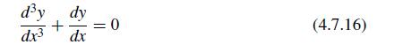
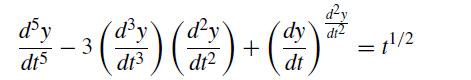
Write the system of first-order equations we need to solvesubject to d³y dy dx3 dx + = 0 (4.7.16)
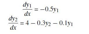
Consider the system of ordinary differential equationswith y1(0) = 4 and y2(0) = 6 and for step size h = 0.5. Find(a) y1(2) and y2(2) using the explicit Euler method(b) y1(0.5) and y2(0.5) using the fourth-order Runge–Kutta method. dy2 dx dy1 = dx –0.5y1 = 4-0.3y2 -0.1y1
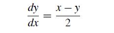
Consider the nonlinear ordinary differential equationwith y(0) = 1. Estimate y(1)(a) Using the explicit Euler’s method with h = 0.2(b) Using the fourth-order Runge–Kutta method with h = 1. dy dx || x-y 2
Convert the second-order ODEinto an autonomous system of ODEs. y" - y² = xy(0) = 2, y (0) = -1
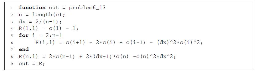
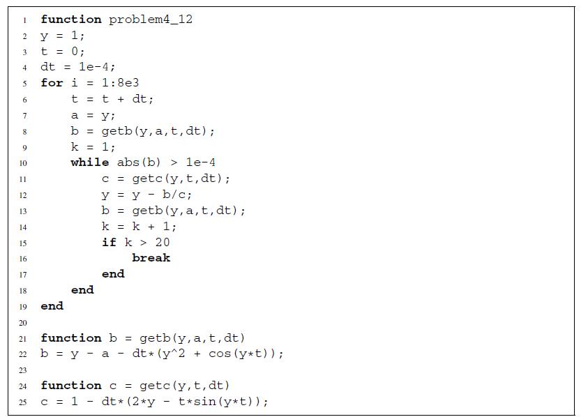
Answer the following questions about this program:(a) What differential equation is solved by this program?(b) What is the initial condition?(c) What does the variable a represent?(d) What does the variable b represent?(e) What does the variable c represent?(f) What numerical method is implemented
Consider the system of equations(a) Calculate the eigenvalues and eigenvectors.(b) Using matrix diagonalization, obtain (analytically) the solution of the equations for y1(0) = y2(0) = 1.(c) How does the solution behave for large t? Is this consistent with your eigenvalue analysis? Explain.(d)
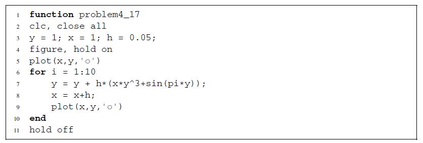
Consider the following MATLAB program:Show that the first step of the integration satisfies the stability criterion. 1 function problem4_17 2 3 4 5 6 7 8 9 clc, close all y = 1; x = 1; h = 0.05; figure, hold on plot (x, y, 'o') for i=1:10 y = y + h* (x*y^3+sin (pi*y)); x = x+h; plot (x, y,
Consider the following system of ordinary differential equationswith y1(0) = 0.5 and y2(0) = 5. We consider the explicit Euler method for numerical integration. What is the maximum value for the time step h that guarantees numerically stable integration over a single time step? Do you expect the
Use a linear stability analysis to determine the maximum step size that you could use for the forward Euler integration of the differential equation y″ + 2(y′)2 − y = 0 as a function of the local slope, y′(x).
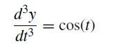
How many coupled first-order IVPs are required to solve the problemusing RK4 with appropriate initial conditions? d³y dt3 = cos(t)
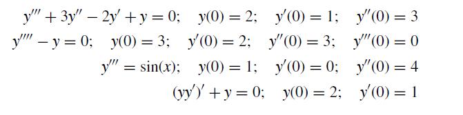
Convert the following higher-order differential equations into a system of autonomous first-order differential equations y"" + 3y" - 2y + y = 0; y(0) = 2; y"" -y=0; y(0) = 3; y(0) = 2; y" sin(x); = y(0) = 1; (yy) +y=0; y(0) = 1; y'(0) = 3; y'(0) = 0; y(0) = 2; y'(0) = 3 y"(0) = 0 y(0) = 4 y(0) = 1
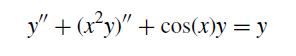
Consider nonlinear ordinary differential equationsubject to initial conditionsConvert this problem into a system of autonomous equations and initial conditions. y" + (x²y)" + cos(x)y = y
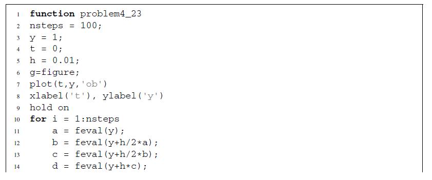
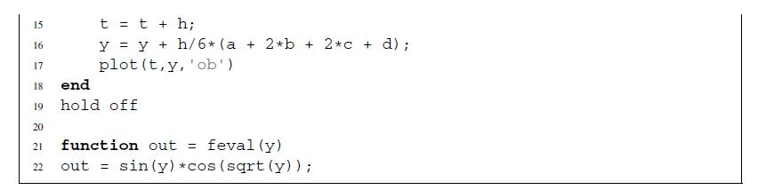
What ODE is solved by the following MATLAB code and what method is used? Include the initial condition in your answer. 1 function problem4_23 2 3 4 nsteps = 100; y = 1; t = 0; h = 0.01; 5 6 g=figure; 7 plot(t, y, 'ob') 8 xlabel('t), ylabel ('y') 9 hold on 10 for i=1:nsteps 11 12 13 14 a =
Consider the solution of the differential equationby an implicit Euler scheme. Determine the form of the residual and Jacobian that you would need to compute the values for time step i + 1. y"+yy + y³ = sin(x); y(0) = 1; y(0) = 2
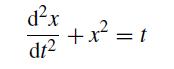
Determine the Jacobian required to integrate the equationusing implicit Euler. x + x - 2x + 3x³ = 0
Consider the nonlinear differential equationsubject to the conditions x = 3 and dx/dt = 2 at the time t = 1. Let’s solve this problem using implicit Euler with a time step of h = 1/2. You may recall that a continuation method is often useful in this problem; you should use x(0)i+1 = xi as the
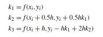
One possible third-order Runge–Kutta method is given bywhereBy analyzing the linear problemdetermine the function f (hλ) appearing in the criterionfor stable integration. You do not need to actually compute the maximum step size, as this would be best done using a computer. What numerical method
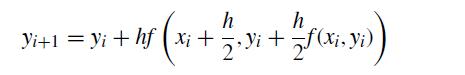
Determine the stability condition for the step size h for the midpoint method, which has the form h h Yi+1 = Yi + hf ( xi + 12 - Yi + 1/ƒ (xi, yi))
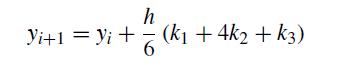
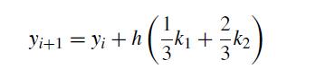
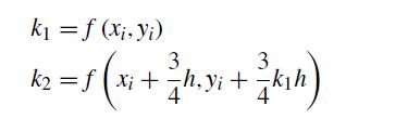
Determine the stability condition for the step size h for Ralston’s method, which has the formwhere Y²₁1 = 3₁+ h (= k₁ + ² k₂) 3
Determine the stability condition for the step size h for the trapezoidal integration method, which has the form h Yi+1=Yi+[f (vi) + f (Vi+1)]
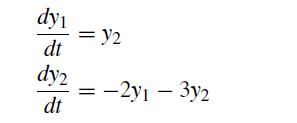
Answer the following seven questions about the program listed below that solves a system of two ODEs for the unknowns y1 and y2.(a) What numerical method is implemented to solve these ordinary differential equations?(b) What system of ordinary differential equations is this program solving?(c) Are
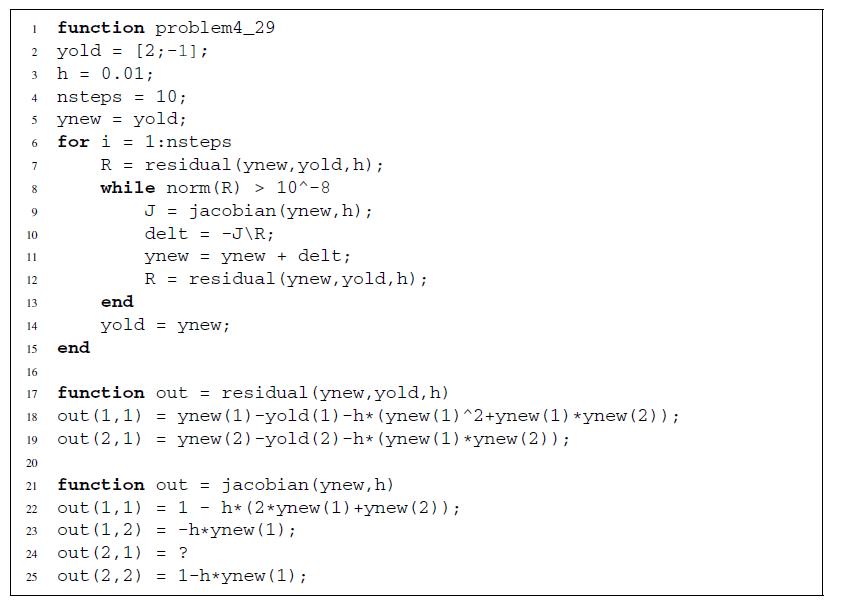
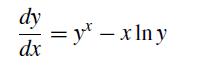
Write a MATLAB program that uses implicit Euler to integrateUse an initial condition y(0) = 1 and integrate until x = 2. What equations are needed for Newton’s method? Is this solution becoming unstable? dy dx = y² - xlny
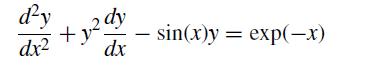
Write a MATLAB program that uses RK4 to solve the ODEsubject to the initial conditions y(0) = 1 and y(0) = 0. You should compute the solution for the step size h = 0.01. Make a plot of the function y(x) over the range x = [0, 10]. d'y dy +y dx dx² - sin(x)y exp(-x) =
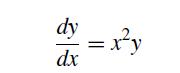
Write a MATLAB program that does an RK4 integration of the differential equationfor the initial condition y(1) = 2 up to a maximum value x = 5. Your program should automatically generate a single plot with a legend that has the evolution of the function y(x) for the step sizes h = 0.2, h = 0.08 and
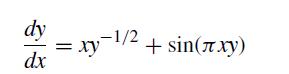
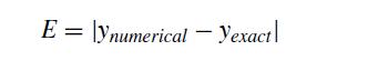
Write a MATLAB program that uses the predictor–corrector method to solve the ODEsubject to the initial condition y(0) = 1. You should compute the solution for the step sizes h = 0.1, 0.01, . . . , 10−7.Make a log–log plot of the absolute error in the numerical solution at the value x = 2 as a
This problem set deals with the Schlögel model for a bistable biochemical reaction. You can read more about it in the paper “On thermodynamics near a steady state” (Z. Physik 248, 446–458, 1971). For our purposes, you can think of the model as being the solution to the ordinary differential
This problem deals with the numerical analysis of the solution toThis is a separable ordinary differential equation with the solutionThe exact solution is denoted as y∗ for future reference.(a) We will begin by looking at the solutions produced by using either explicit Euler or RK4 and comparing
Consider the ordinary differential equation from Problem 4.32 but with a new initial condition, y(1) = 1. What is the largest step size, h∗, in RK4 such that the system is stable for the first step? Rename your program from Problem 4.32 and modify the parameters so that it produces a solution for
In this problem, you are going to look at how the accuracy of the solution of an ODE depends on the time step. Consider the integration of the differential equationover the domain x ∈ [0, 1] with the initial condition y(0) = 0. Write a program that uses implicit Euler to compute the value of y(1)
In this problem, you are going to use RK4 to find the minimum value of the solution of a third-order ordinary differential equation. Consider the solution of the differential equationsubject to the initial conditionsover the domain x ∈ [0, 1]. You should write a MATLAB program that uses a
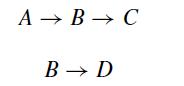
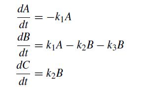
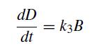
Determine the solution to the kinetic systemwhere the reaction rates are k1, k2, and k3 (in the order written here). The corresponding ODEs that you need to solve areThe initial condition is a concentration A0 and no B, C, or D.Write a MATLAB program that plots the solution up to t = 10 for k1 = 2,
Use RK4 to find the solution tosubject to the initial conditions y(0) = −1, y′(0) = 1/2, y″(0) = −1/3, y″′= 1/4, and y″″ = −1/5. Your program should make a plot of the fourth derivative of y versus the second derivative of y up to a time t = 1. What equations convert this into an
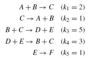
Consider the set of reactions and rate constantswith an initial concentration of 0.75 moles of A and 1 mole of B. Write the system of ordinary differential equations describing the concentration of each species, along with appropriate initial conditions. Numerically integrate this system out to t =
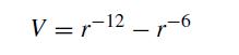
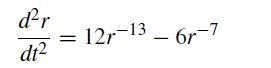
Consider two particles that are interacting via a Lennard–Jones potential,The dynamic equation for the distance r between these particles is given by the force balance (in dimensionless form),where we used the relationship between potential energy and force, f = −dV/dr. Write a MATLAB program
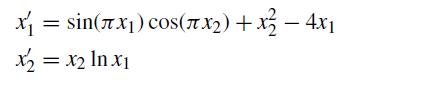
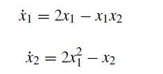
Perform a linear stability analysis of the systemabout the steady state x1 = 1 and x2 = 2. What type of steady state do you find? Ix-x+ (x²)soo (x2) = x x₂ = x2 In x₁
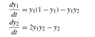
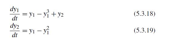
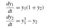
Analyze the stability and the nature of the nearby trajectories for the steady states of dyi dt dy2 dt = y1 - y + y₂ = y1 - yi (5.3.18) (5.3.19)
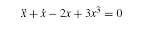
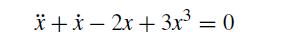
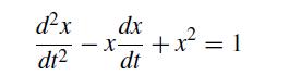
Consider the dynamics of the damped, forced oscillatorClassify the steady states in the position/velocity phase space (x, ˙x). x + x - 2x + 3x³ = 0
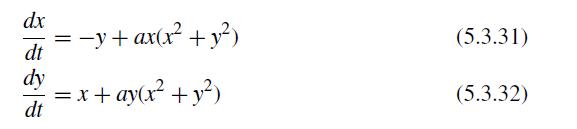
Analyze the stability and the nature of the nearby trajectories for the steady states ofwhere a is a constant. dx dt dy dt = -y + ax(x² + y²) = x + ay(x² + y²) (5.3.31) (5.3.32)
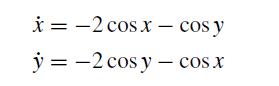
Consider the dynamical systemWhat type of steady state (or steady states) are nearest to the origin? x = -2 cosx- cos y y=-2 cos y cos.x
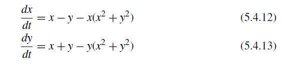
Analyze the phase plane trajectories for the system dx == x - y - x(x² + y²) dt dy dt = x + y − y(x² + y²) (5.4.12) (5.4.13)
Classify the two steady states of the dynamic system and make a sketch of the phase plane near the steady states for the systemYour phase plane only needs to show the basic idea and you do not need to worry about the directions of the eigenvectors or the sense of rotation. dy1 dt dy2 dt = y₁ -
Analyze the phase plane trajectories for the system dx dt dy dt = -y + x(p-x² - y²) = x + y(p-x² - y²) (5.5.7) (5.5.8)
Use linear stability analysis to make a sketch of the phase plane for et²-y² - 1 []=[²²] x²y-¹ +2 dt
Consider the force balance for the position x of a particle subject to the following force balanceSketch the phase plane where the x-axis is the position and the y-axis is the velocity. dt a+zx 1 = a + : dx - TIP d²x
Is the steady state at (x1 = 0, x2 = 0) forstable, neutrally stable, or unstable? 1x - x = 7x Ix - 7x¹x = ¹x X₁
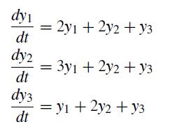
Determine the stability of the steady state solution of dy₁ dt dy2 dt dy3 dt 2y1 + 2y2 + y3 3y1 + 2y2 + y3 = y1 + 2y2 + Y3
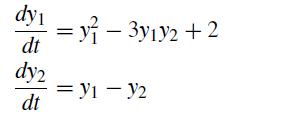
Consider the system of equations(a) Is the steady state at (y1 = 0, y2 = 0) stable, unstable, or neutrally stable?(b) Solve this system corresponding to the initial conditions y1(0) = 0 and y2(0) = 1.(c) Explain why the steady state solution to part (b) does not agree with the answer to part (a).
Consider the dynamic systemsubject to the initial conditions x(0) = 1 and y(0) = 1. What are the steady state values of x and y for this system of equations? (b) What are the eigenvalues for this system of equations? Consider the numerical integration of this system of equations where you start
How do the location and classifications of the steady states for the systemchange if the second equation becomes [x2] = [ d dt X2 x² + x2 x1 + x2
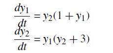
For the dynamical system(a) Calculate the steady state values of y1, y2.(b) For each steady state, calculate the eigenvalues and assess its stability.(c) Provide sketches of the corresponding phase plane plots, indicating clearly their key features. dy1 dt dy2 dt = y2(1 + y₁) =Y1()2+3)
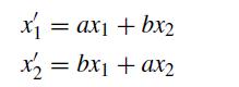
Perform a linear stability analysis of the systemaround the steady state solution. How does the approach to the steady state depend on the parameters a and b? x₁ = ax₁ + bx₂ x₂ = bx₁ + ax₂
Consider a system of equations with a steady state Jacobian ofwhere a is some rational number. For what values of a is the steady state a saddle point? J 13 - [18] a 0
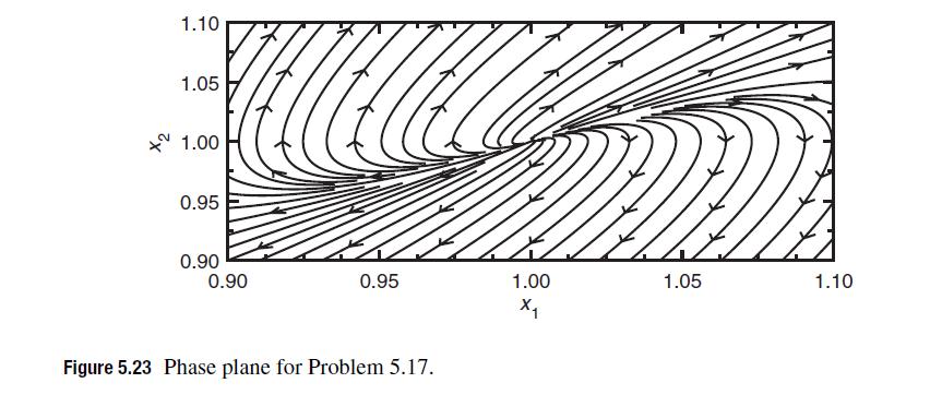
The systemhas a steady state at (x1 = 1, x2 = 1). You can analyze this steady state using linear stability analysis, or just consider the phase plane in Fig. 5.23. What can you say about the real and imaginary parts of the eigenvalues of the steady state Jacobian for this problem? You can provide a
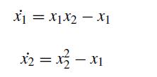
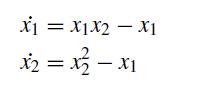
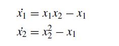
Consider the nonlinear system of ODEsIf we want to perform a linear stability analysis at some point in the solution corresponding to x1 and x2, what is the Jacobian that we need for this system of equations? Ix - 7x¹x = 1x x2 = x² - x1
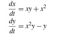
Consider the system of ordinary differential equations(a) Confirm that (x,y) = (0,0), (1,−1), and (−1,1) are steady states of this system.(b) What is the 2 × 2 steady state Jacobian for this system in terms of x and y?(c) Determine the stability and the classification (node, spiral, saddle
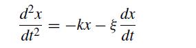
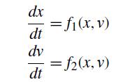
Consider the force balance for a damped harmonic oscillator with mass m = 1 kg, a spring constant k > 0 in N/m, and a friction coefficient ξ > 0 in kg/s,subject to some initial position x0 and initial velocity v0.(a) Define the right-hand-side functions f1 and f2 and state the initial
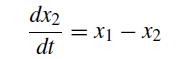
Consider the system of equationsDetermine the stability of the steady states of these equations and sketch the phase plane. Confirm that your sketch is qualitatively correct by integrating these equations using RK4 with initial guesses x1 = 0.01, x2 = −5 and x1 = −0.01, x2 = −5. Do you feel
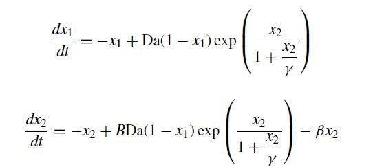
Uppal, Ray, and Poore provide the following system of differential equations describing irreversible, first-order, exothermic reactions in a CSTR:where x1 and x2 are dimensionless concentration and temperature variables respectively, and Da, γ , B, and β are dimensionless parameters that describe
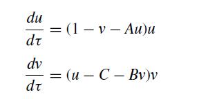
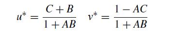
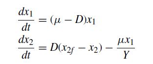
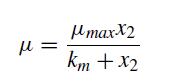
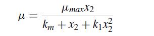
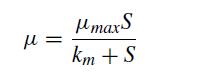
Consider a bioreactor described by the set of balance equationswhere x1 and x2 represent the biomass and substrate concentrations in the reactor. The growth rate depends on the substrate concentration. Different models have been proposed to represent this dependance.• Monod kinetics:• Substrate
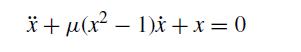
The van der Pol equation iswhere μ is a parameter. This system exhibits a limit cycle in the plane (x, ˙x) (i.e., in momentum-position phase space). For the parameter μ = 1.1, write a MATLAB program that uses numerical integration to determine whether this is a stable limit cycle or an unstable
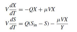
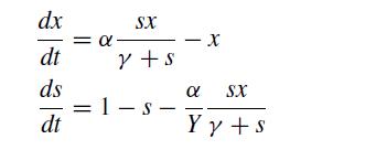
In this problem, we will analyze a dynamic model of the two-species CSTR bioreactor shown in Fig. 5.24. On the left, fresh media with a substrate concentration Sin enters at a volumetric flow rate Q. Inside the reactor volume V, bacteria at a concentration X consume the substrate at concentration S
Consider the dynamical system(a) Use linear stability analysis to characterize the steady states in the interval x ∈ [−3.5, 3.5] and y ∈ [−3.5, 3.5]. You are not allowed to use the eigenvalue functions in MATLAB to compute the eigenvalues but you can use this function to check your
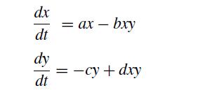
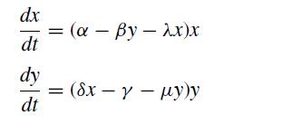
Consider a simple predator–prey modelwith parameters a = 1.2, b = 0.6, c = 0.8, and d = 0.3. Employ initial conditions of x(0) = 2 and y(0) = 1 and integrate numerically from t = 0 to 30. Compare the performance of explicit Euler and Runge–Kutta fourth-order method for a time step of Δt =
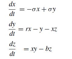
Consider the Lorenz equationswith parameters σ = 10, b = 8/3, and r = 28. Employ initial conditions of x(0) = y(0) = z(0) = 5 and integrate from t = 0 to 20. Use the Runge–Kutta fourth-order method for the integration with a time step of Δt = 0.031 25.(a) For the above initial condition
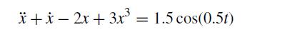
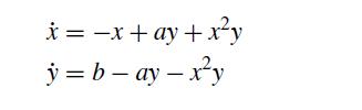
Consider the equation(a) Write a MATLAB program that produces the phase plane. You are welcome to use any integration method you would like. The phase plane portrait that you make should be wide enough to show all of the steady states. Explain why you do (or do not) see the behavior predicted by a
In this problem, you will use your knowledge of solving systems of ordinary differential equations and phase planes to look at the classic predator–prey problem in biology. The model itself is very simple and covered in numerous textbooks on biology, population dynamics, and nonlinear analysis.
In this problem, you will use your knowledge of the phase plane and stability to analyze a simple model of glycolysis. The glycolysis pathway that first convert glucose into fructose-6-phosphate (F6P), and later lead to two molecules of pyruvate, which then enters the TCA cycle. In the course of
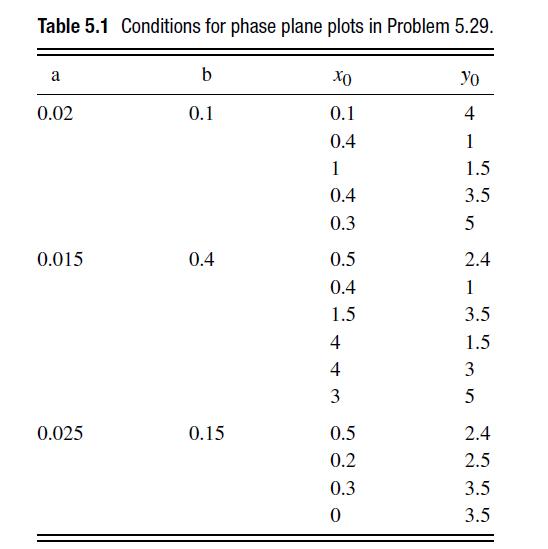
In this problem, we will look at the phase plane dynamics of a particle in a doublewell potential given by the dynamic equationThe term on the left-hand side is the acceleration, and the term on the right-hand side is the force due to a potentialIf you plot the potential, you will see that it has a
What is the grid spacing Δx if you discretize the space x ∈ [−1, 1] with 51 nodes?
Derive a centered finite difference formula for the second derivative using four evaluation points.
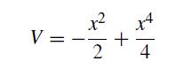
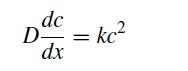
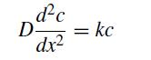
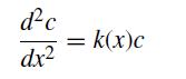
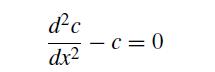
Show how the error in the finite difference approximation depends on the number of nodes n for the reaction–diffusion equation.with c(0) = 0 and c(1) = 1. In chemical engineering lingo, the quantity ϕ is the Thiele modulus for this problem. d²c = p²c dx² (6.3.3)
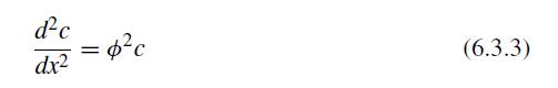
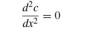
Consider the same ODE as in Example 6.3 but use a Neumann boundary condition on the left boundary, e.g.,Example 6.3Develop a MATLAB code to solvefor an arbitrary number of nodes. dy dx |x=-1 = 10 (6.3.29)
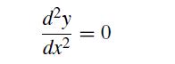
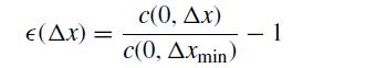
What is the equation for c1 for the solution of the diffusion equation d2c/dx2 = 0 with a no-flux boundary condition at the left boundary?
Develop a MATLAB code to solvefor an arbitrary number of nodes. d²y dx² = -2y(1-2y²), y(-1)=-1, y(1) = 1 (6.3.15)
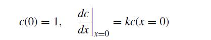
In a one-dimensional boundary value problem with a no-flux condition on the left boundary, what is the relationship between the fictitious node and the nodes in the domain?
Consider a coupled system of boundary value problems for x and y. If the unknowns are in a vector z in an order that preserves the band structure, what are the first five entries in z?
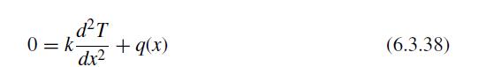
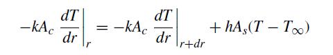
Consider the solid bar in Figure 6.7. The temperature of the bar is maintained at the constant value T0 at the boundaries x = −1 and x = 1. In the middle of the bar, from a region −ϵ where k is the thermal conductivity and q(x) is the position-dependent heat generation rate termCompute the
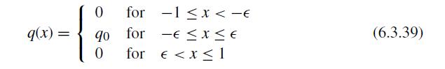
Use Taylor series expansions to derive the centered finite difference formula for the third derivative, d³y Yi+22yi+1 + 2yi-1 - Yi-2 dx3 2(Δ.x)3
Use the problem in Example 6.2 with ϕ = 1 to illustrate mesh refinement from n = 3 to n = 7.Example 6.2Show how the error in the finite difference approximation depends on the number of nodes n for the reaction–diffusion equation.with c(0) = 0 and c(1) = 1. In chemical engineering lingo, the
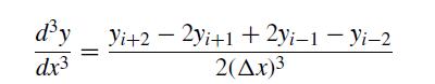
The centered finite difference formulas can be written in the formwhere k is the order of the derivative and the values of j denote locations relative to node i. For this problem, we will consider the lowest-order form for the fourth derivative using the Taylor series approach.(a) Write out the
Determine the residual and Jacobian needed to solve the equationsubject to y(0) = 1 and y(1) = 0 using centered finite differences and n = 5 nodes. (yy) = √y
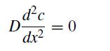
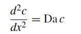
Determine the residual and Jacobian needed to solve the diffusion equation,subject to c(0) = 1 on the left boundary and a second-order depletion reaction,on the right boundary using centered finite differences and n = 4 nodes. d²c D = 0 dx²
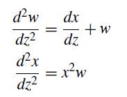
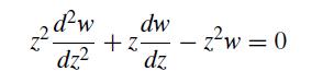
Consider the centered finite difference solution of the coupled system of equationsusing four nodes. Discretize the differential equations for w3 and x3 and then rewrite these equations in terms of a single variable y that interleaves the variables w and x. d²w dz² d²x C dz² || dx dz || + w M_X
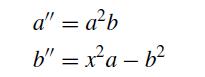
Consider the coupled system of second-order differential equationssubject to a(0) = 1, a′(1) = 2, b′(0) = 0 and b(1) = 1. Define a single system of unknowns y = [a1, b1, a2, b2, . . .] to solve this system by finite differences. You do not need to convert this into an autonomous system of
We can get an accurate idea of the error in centered finite differences by studying the solution to an exactly solvable problem and directly calculating the error in the finite difference representation. Consider the simple reaction–diffusion problemwhere Da is the Dämkohler number. (We have
In the course of solving a boundary value problem for some function c(x) using centered finite differences, there is a subfunction for computing the residuals that has the following structure:Answer the following questions about this problem.(a) If x1 = 0, what is xn?(b) What is the ordinary
Write a MATLAB program that solves the diffusion equationsubject to the boundary conditions y(0) = 1 and dy/dx = −y3/2 at x = 1 using finite centered differences. Show that your numerical result agrees with the analytical solution to this nonlinear problem by plotting both results together. d-y
Consider the solution to the reaction diffusion equationwith boundary conditions c(0) = 1 and c(L) = 0. Write a MATLAB program that uses centered finite differences to solve this equation for Da = kL2/D values of 0.01, 0.1, 1, 10, 100, 1000. Your program should be written so that you specify an
In this problem, we will look at the convergence of the solution to a boundary value problem as a function of the grid spacing. Consider the reaction–diffusion equationwhere the spatially dependent reaction term isThe boundary conditions for the problem are c(−1) = 1 and c(1) = 0.5.You should
Write a MATLAB code to solve the diffusion equationover the domain x ∈ [0, 1] subject tofor the (dimensionless) reaction rate k = 2. Your program should plot the solution and compare the result to the exact solution of this linear problem. Include the derivation of the exact result along with a
Consider the equation(a) Write a MATLAB program that solves the diffusion–reaction problem on the domain x ∈ [0, 0.5] subject to c(0) = 1 and c(0.5) = 0. Your program should generate two plots: (i) the numerical solution and the exact solution for Δx = 0.01 and (ii) the norm of the difference
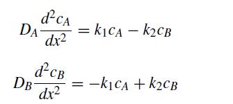
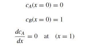
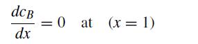
This problem consists of three numerical calculations that involve the coupled reaction–diffusion systemwhere DA and DB are the diffusion coefficients for species A and B, respectively, and k1 and k2 are reaction rates. The boundary conditions for these equations areYou will write three
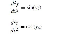
Write a MATLAB program that uses finite differences to solveover the interval x ∈ [0, π]. The boundary conditions at x = 0 are y = z = 1 and the boundary conditions at x = π are y = z = 0. Your program should automatically generate a plot of y versus x and z versus x.
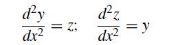
Write a MATLAB code to solve the coupled systemon the domain x ∈ [0, 1] subject to y(0) = 1, y(1) = 2, z(0) = 0, and z(1) = 2. Your program should use the optimal band structure for this problem and plot the solution. Include the finite difference equations used in your program. Ap zxp
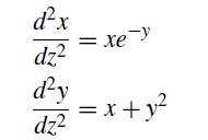
Write a MATLAB program that solves the coupled system of equationssubject to x(1) = 0.8, y(1) = 1, dx/dz = 0 at z = 0, and dy/dz = x at z = 0 using interleaved variables. Your program should generate a plot of x(z) and y(z). d²x dz² d'y dz² = xey = x+y²
This problem concerns the solution of heat transfer from a radial fin. Although this problem has a solution in terms of Bessel functions, we are going to see how to compute it numerically directly from the boundary value problem.(a) Consider a radial fin of thickness t and length L. The fin has a
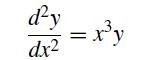
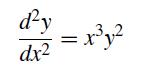
Write a MATLAB program that uses finite difference to solveon x ∈ [0, 1] subject to y(0) = 1 and y′(1) = 0 andon x ∈ [0, 1] subject to y(0) = 1 and y′(1) = 0. Use the solution to the linear problem, y″ = x3y as the initial guess. Your program should plot the solutions to both the linear
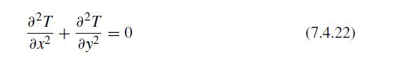
Write a MATLAB program to solvein a square boundary subject to n · ∇T = 0 on all of the sides except the top, where T = 0. There is a hot spot in the center corresponding to T(0.5, 0.5) = 1. Note that we have already converted this problem into dimensionless form. а 2 т ах2 а 2
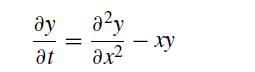
Write the ordinary differential equation for an interior node produced by the method of lines for the PDE ду at Aze 2x2 - ху
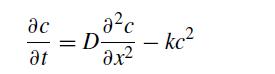
Consider the method of lines solutions of the unsteady reaction–diffusion equation with a second-order bulk reaction,with an initial concentration c = 0 and boundary conditions c(0) = 1 and ∂c/∂x = 0 at x = L. Answer the following questions.(a) If we discretize with centered finite

Showing 200 - 300 of 375

1
2
3
4

Step by Step Answers

Services

Sitemap
Fun
Definitions
Become Tutor
Used Textbooks
Study Help Categories
Recent Questions
Expert Questions
Campus Wear
Sell Your Books

Company Info

Security
Copyrights
Privacy Policy
Terms & Conditions
SolutionInn Fee
Scholarship
Online Quiz
Give Feedback, Get Rewards

Get In Touch

About Us
Contact Us
Career
Jobs
FAQ
Student Discount
Campus Ambassador

Secure Payment

Download Our App

© 2026 SolutionInn. All Rights Reserved