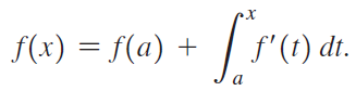
New Semester Started Get 50% OFF Study Help! --h --m --s Claim Now

Question Answers

Textbooks

Find textbooks, questions and answers

Oops, something went wrong!

Change your search query and then try again

Result Not Found

Books FREE
Study Help
Tutors
AI Study Planner NEW
Sell Books

Search
Sign In
Register

study help
mathematics
calculus early transcendentals

Calculus Early Transcendentals 2nd edition William L. Briggs, Lyle Cochran, Bernard Gillett - Solutions

Graph the following spirals. Indicate the direction in which the spiral is generated as θ increases, where θ > 0. Let a = 1 and a = -1.Logarithmic spiral: r = eaθ
Graph the following spirals. Indicate the direction in which the spiral is generated as θ increases, where θ > 0. Let a = 1 and a = -1.Spiral of Archimedes: r = aθ
Show that the graph of r = a sin mθ or r = a cos mθ is a rose with m leaves if m is an odd integer and a rose with 2m leaves if m is an even integer.
Equations of the form r = a sin mθ or r = a cos mθ, where a is a real number and m is a positive integer, have graphs known as roses. Graph the following roses.r = 6 sin 5θ
Equations of the form r = a sin mθ or r = a cos mθ, where a is a real number and m is a positive integer, have graphs known as roses. Graph the following roses.r = 2 sin 4θ
Equations of the form r = a sin mθ or r = a cos mθ, where a is a real number and m is a positive integer, have graphs known as roses. Graph the following roses.r = 4 cos 3θ
Equations of the form r = a sin mθ or r = a cos mθ, where a is a real number and m is a positive integer, have graphs known as roses. Graph the following roses.r = sin 2θ
Equations of the form r2 = a sin 2θ and r2 = a cos 2θ describe lemniscates. Graph the following lemniscates.r2 = -8 cos 2θ
Equations of the form r2 = a sin 2θ and r2 = a cos 2θ describe lemniscates. Graph the following lemniscates.r2 = -2 sin 2θ
Equations of the form r2 = a sin 2θ and r2 = a cos 2θ describe lemniscates. Graph the following lemniscates.r2 = 4 sin 2θ
Equations of the form r2 = a sin 2θ and r2 = a cos 2θ describe lemniscates. Graph the following lemniscates.r2 = cos 2θ
Consider the family of limaçons r = 1 + b cos θ. Describe how the curves change as b→∞.
The equations r = a + b cos θ and r = a + b sin θ describe curves known as limaçons (from Latin for snail). We have already encountered cardioids, which occur when |a| = |b|. The limaçon has an inner loop if |a| < |b|. The limaçon has a dent or dimple if |b| < |a| < 2|b|. And the
Use the result of Exercise 84 to describe and graph the following lines.r(4 sin θ - 3 cos θ) = 6
Use the result of Exercise 84 to describe and graph the following lines.r(sin θ - 4 cos θ) - 3 = 0
Use the result of Exercise 84 to describe and graph the following lines.r cos (θ + π/6) = 4
Use the result of Exercise 84 to describe and graph the following lines.r cos (π/3 - θ) = 3
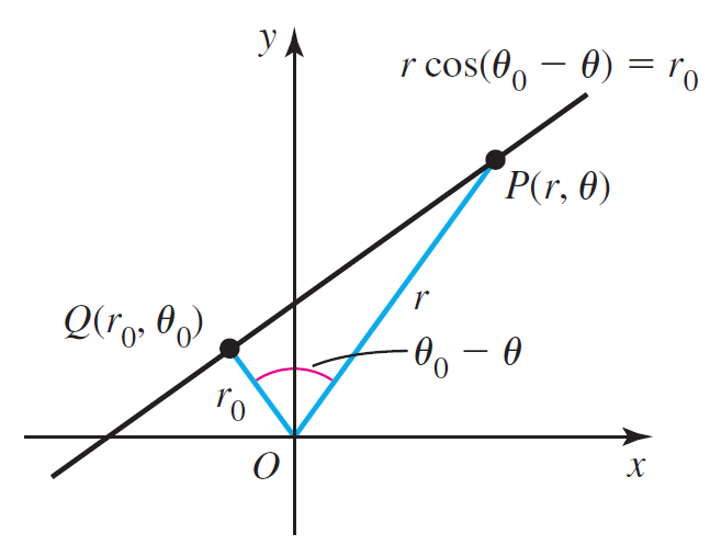
a. Show that an equation of the line y = mx + b in polar coordinates is r = b/sin θ - m cos θ.b. Use the figure to find an alternative polar equation of a line, r cos (θ0 - θ) = r0. Note that Q(r0, θ0) is a fixed point on the line such that OQ is perpendicular to the line and r0 ≥ 0; P(r,
Consider the polar curve r = 2 sec θ.a. Graph the curve on the intervals (π/2, 3π/2), (3π/2, 5π/2), and (5π/2, 7π/2). In each case, state the direction in which the curve is generated as θ increases.b. Show that on any interval (nπ/2, (n + 2)π/2), where n is an odd integer, the graph is
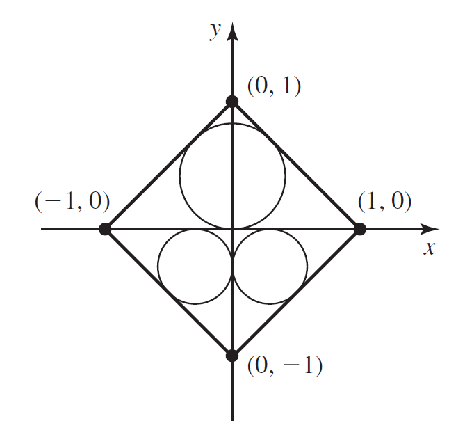
Find equations of the circles in the figure. Determine whether the combined area of the circles is greater than or less than the area of the region inside the square but outside the circles. y. УА (0, 1) (-1, 0) (1, 0) х (0, – 1)
Use the results of Exercises 74–75 to describe and graph the following circles.r2 - 2r(-cos θ + 2 sin θ) = 4
Use the results of Exercises 74–75 to describe and graph the following circles.r2 + 2r(cos θ - 3 sin θ) = 4
Use the results of Exercises 74–75 to describe and graph the following circles.r2 - 2r(2 cos θ + 3 sin θ) = 3
Use the results of Exercises 74–75 to describe and graph the following circles.r2 - 8r cos (θ - π/2) = 9
Use the results of Exercises 74–75 to describe and graph the following circles.r2 - 4r cos (θ - π/3) = 12
Use the results of Exercises 74–75 to describe and graph the following circles.r2 - 6r cos θ = 16
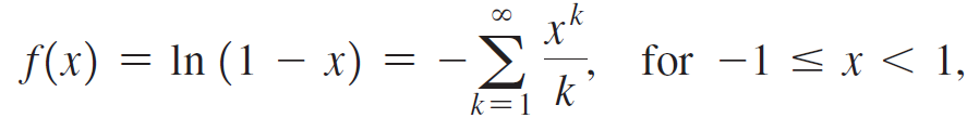
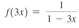
Use the power series representationto find the power series for the following functions (centered at 0). Give the interval of convergence of the new series.f(3x) = ln (1 - 3x) f(x) = In (1 - x) = - > for -1 < x < 1, k' k=1 8.
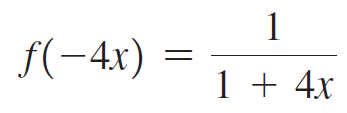
Use the geometric seriesto find the power series representation for the following functions ( centered at 0). Give the interval of convergence of the new series. Ex, for |x| < 1, f(x) k=0 8. || f(-4x) 1 + 4x
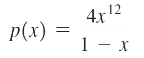
Use the geometric seriesto find the power series representation for the following functions ( centered at 0). Give the interval of convergence of the new series. Ex, for |x| < 1, f(x) k=0 8. || 4x12 p(x) 1 — х
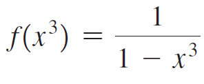
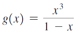
Use the geometric seriesto find the power series representation for the following functions ( centered at 0). Give the interval of convergence of the new series. Ex, for |x| < 1, f(x) k=0 8. || f(x³) = 1 — х3 ||
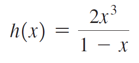
Use the geometric seriesto find the power series representation for the following functions ( centered at 0). Give the interval of convergence of the new series. Ex, for |x| < 1, f(x) k=0 8. || 2x3 h(x) 1 — х
Use the geometric seriesto find the power series representation for the following functions ( centered at 0). Give the interval of convergence of the new series. Ex, for |x| < 1, f(x) k=0 8. || 8(х) +3 1 — х
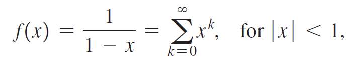
Use the geometric seriesto find the power series representation for the following functions ( centered at 0). Give the interval of convergence of the new series. Ex, for |x| < 1, f(x) k=0 8. ||
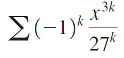
Determine the radius of convergence of the following power series. Then test the endpoints to determine the interval of convergence. Σ-) 27k
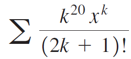
Determine the radius of convergence of the following power series. Then test the endpoints to determine the interval of convergence. k 20 xk (2k + 1)!
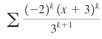
Determine the radius of convergence of the following power series. Then test the endpoints to determine the interval of convergence. (-2)* (x + 3)* Σ 3k+1
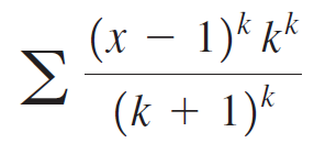
Determine the radius of convergence of the following power series. Then test the endpoints to determine the interval of convergence. (x – 1)* kk Σ (k + 1)k
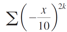
Determine the radius of convergence of the following power series. Then test the endpoints to determine the interval of convergence. 2k 10
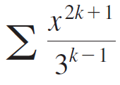
Determine the radius of convergence of the following power series. Then test the endpoints to determine the interval of convergence. x2k +1 3k–1
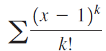
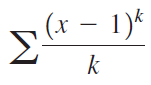
Determine the radius of convergence of the following power series. Then test the endpoints to determine the interval of convergence.∑ k (x - 1)k
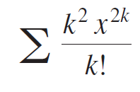
Determine the radius of convergence of the following power series. Then test the endpoints to determine the interval of convergence. k2 x2k k!
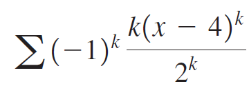
Determine the radius of convergence of the following power series. Then test the endpoints to determine the interval of convergence. k(x – 4)* 2k
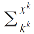
Determine the radius of convergence of the following power series. Then test the endpoints to determine the interval of convergence. _k
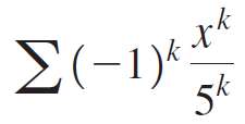
Determine the radius of convergence of the following power series. Then test the endpoints to determine the interval of convergence. Σ(-1) μt 5k
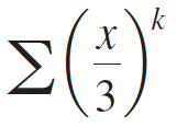
Determine the radius of convergence of the following power series. Then test the endpoints to determine the interval of convergence. k 3
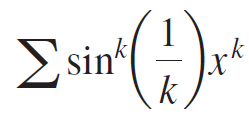
Determine the radius of convergence of the following power series. Then test the endpoints to determine the interval of convergence. 2sink
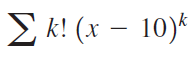
Determine the radius of convergence of the following power series. Then test the endpoints to determine the interval of convergence. ΣΗ (- 0)* 10)* k!
Determine the radius of convergence of the following power series. Then test the endpoints to determine the interval of convergence.∑(kx)k
Determine the radius of convergence of the following power series. Then test the endpoints to determine the interval of convergence.
Determine the radius of convergence of the following power series. Then test the endpoints to determine the interval of convergence. (x – 1)* Σ k!
Determine the radius of convergence of the following power series. Then test the endpoints to determine the interval of convergence. , (x – 1)* ΣΗ
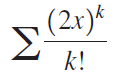
Determine the radius of convergence of the following power series. Then test the endpoints to determine the interval of convergence. (2x)* k!
Determine the radius of convergence of the following power series. Then test the endpoints to determine the interval of convergence.∑(2x)k
How are the radii of convergence of the power series ∑ck xk and ∑(-1)k ck xk related?
What is the interval of convergence of the power series ∑(4x)k?
What is the radius of convergence of the power series ∑ck (x/2)k if the radius of convergence of ∑ck xk is R?
Do the interval and radius of convergence of a power series change when the series is differentiated or integrated? Explain.
Explain why a power series is tested for absolute convergence.
What tests are used to determine the radius of convergence of a power series?
Write the first four terms of a power series with coefficients c0, c1, c2, and c3 centered at 3.
Write the first four terms of a power series with coefficients c0, c1, c2, and c3 centered at 0.
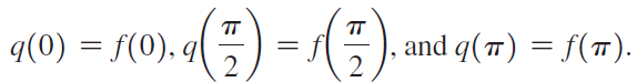
When approximating a function f using a Taylor polynomial, we use information about f and its derivatives at one point. An alternative approach (called interpolation) uses information about f at several different points. Suppose we wish to approximate f(x) = sin x on the interval [0, π].a. Write
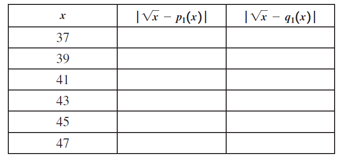
Let p1 and q1 be the first-order Taylor polynomials for f(x) = √x centered at 36 and 49, respectively.a. Find p1 and q1.b. Complete the following table showing the errors when using p1 and q1 to approximate f(x) at x = 37, 39, 41, 43, 45, and 47. Use a calculator to obtain an exact value of
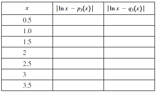
Let f(x) = ln x and let pn and qn be the nthorder Taylor polynomials for f centered at 1 and e, respectively. a. Find p3 and q3.b. Graph f, p3, and q3 on the interval [0, 4].c. Complete the following table showing the errors in the approximations given by p3 and q3 at selected points.d.
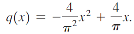
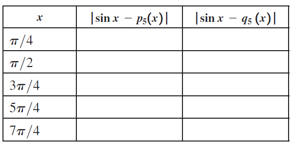
Let f(x) = sin x and let pn and qn be nth order Taylor polynomials for f centered at 0 and π, respectively. a. Find p5 and q5.b. Graph f, p5, and q5 on the interval [-π, 2π]. On what interval is p5 a better approximation to f than q5? On what interval is q5 a better approximation to f than
Suppose f has continuous first and second derivatives at a.a. Show that if f has a local maximum at a, then the Taylor polynomial p2 centered at a also has a local maximum at a.b. Show that if f has a local minimum at a, then the Taylor polynomial p2 centered at a also has a local minimum at a.c.
Let f be differentiable at x = a.a. Find the equation of the line tangent to the curve y = f(x) at (a, f(a)).b. Verify that the Taylor polynomial p1 centered at a describes the tangent line found in part (a).
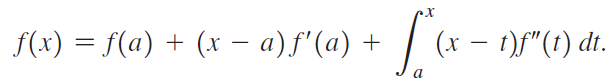
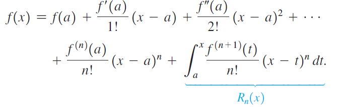
There are several proofs of Taylor’s Theorem, which lead to various forms of the remainder. The following proof is instructive because it leads to two different forms of the remainder and it relies on the Fundamental Theorem of Calculus, integration by parts, and the Mean Value Theorem for
Suppose you wish to approximate e0.35 using Taylor polynomials. Is the approximation more accurate if you use Taylor polynomials centered at 0 or ln 2? Use a calculator for numerical experiments and check for consistency with Theorem 9.2. Does the answer depend on the order of the polynomial?
Suppose you wish to approximate cos (π/12) using Taylor polynomials. Is the approximation more accurate if you use Taylor polynomials centered at 0 or π/6? Use a calculator for numerical experiments and check for consistency with Theorem 9.2. Does the answer depend on the order of the polynomial?
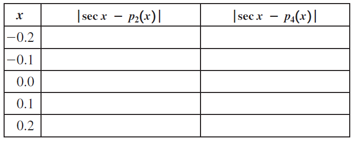
Suppose you approximate f(x) = sec x at the points x = -0.2, -0.1, 0.0, 0.1, and 0.2 using the Taylor polynomials p2(x) = 1 + x2/2 and p4(x) = 1 + x2/2 + 5x4/24. Assume that the exact value of sec x is given by a calculator. a. Complete the table showing the absolute errors in the
Consider the following common approximations when x is near zero.a. Estimate f(0.1) and give a bound on the error in the approximation.b. Estimate f(0.2) and give a bound on the error in the approximation.f(x) = sin-1x ≈ x
Consider the following common approximations when x is near zero.a. Estimate f(0.1) and give a bound on the error in the approximation.b. Estimate f(0.2) and give a bound on the error in the approximation.f(x) = ex ≈ 1 + x
Consider the following common approximations when x is near zero.a. Estimate f(0.1) and give a bound on the error in the approximation.b. Estimate f(0.2) and give a bound on the error in the approximation.f(x) = ln (1 + x) ≈ x - x2/2
Consider the following common approximations when x is near zero.a. Estimate f(0.1) and give a bound on the error in the approximation.b. Estimate f(0.2) and give a bound on the error in the approximation.f(x) = √1 + x ≈ 1 + x/2
Consider the following common approximations when x is near zero.a. Estimate f(0.1) and give a bound on the error in the approximation.b. Estimate f(0.2) and give a bound on the error in the approximation.f(x) = tan-1x ≈ x
Consider the following common approximations when x is near zero.a. Estimate f(0.1) and give a bound on the error in the approximation.b. Estimate f(0.2) and give a bound on the error in the approximation.f(x) = cos x ≈ 1 - x2/2
Consider the following common approximations when x is near zero.a. Estimate f(0.1) and give a bound on the error in the approximation.b. Estimate f(0.2) and give a bound on the error in the approximation.f(x) = tan x ≈ x
Consider the following common approximations when x is near zero.a. Estimate f(0.1) and give a bound on the error in the approximation.b. Estimate f(0.2) and give a bound on the error in the approximation.f(x) = sin x ≈ x
Consider f(x) = ln (1 - x) and its Taylor polynomials given in Example 8. a. Graph y =|f(x) - p2(x)| and y = |f(x) - p3(x)| on the interval [-1/2, 1/2] (two curves).b. At what points of [-1/2, 1/2] is the error largest? Smallest?c. Are these results consistent with the theoretical error bounds
Match functions a–f with Taylor polynomials A–F (all centered at 0). Give reasons for your choices.a. √1 + 2x A. p2(x) = 1 + 2x + 2x2b. 1/√1 + 2x B. p2(x) = 1 - 6x + 24x2c. e2x
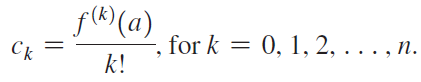
Follow the procedure in the text to show that the nth-order Taylor polynomial that matches f and its derivatives up to order n at a has coefficients f(R) (a) 3D 0, 1, 2, ...,п. for k k! Ск
Determine whether the following statements are true and give an explanation or counterexample.a. Only even powers of x appear in the Taylor polynomials for f(x) = e-2x centered at 0.b. Let f(x) = x5 - 1. The Taylor polynomial for f of order 10 centered at 0 is f itself.c. Only even powers of x
What is the minimum order of the Taylor polynomial required to approximate the following quantities with an absolute error no greater than 10-3?1/√0.85
What is the minimum order of the Taylor polynomial required to approximate the following quantities with an absolute error no greater than 10-3?√1.06
What is the minimum order of the Taylor polynomial required to approximate the following quantities with an absolute error no greater than 10-3?ln 0.85
What is the minimum order of the Taylor polynomial required to approximate the following quantities with an absolute error no greater than 10-3?cos (-0.25)
What is the minimum order of the Taylor polynomial required to approximate the following quantities with an absolute error no greater than 10-3?sin 0.2
What is the minimum order of the Taylor polynomial required to approximate the following quantities with an absolute error no greater than 10-3?e-0.5
Use the remainder to find a bound on the error in the following approximations on the given interval. Error bounds are not unique.√1 + x ≈ 1 + x/2 on [-0.1, 0.1]
Use the remainder to find a bound on the error in the following approximations on the given interval. Error bounds are not unique.ln (1 + x) ≈ x - x2/2 on [-0.2, 0.2]
Use the remainder to find a bound on the error in the following approximations on the given interval. Error bounds are not unique.tan x ≈ x on [-π/6, π/6]
Use the remainder to find a bound on the error in the following approximations on the given interval. Error bounds are not unique.ex ≈ 1 + x + x2/2 on [-1/2, 1/2]
Use the remainder to find a bound on the error in the following approximations on the given interval. Error bounds are not unique.cos x ≈ 1 - x2/2 on [-π/4, π/4]
Use the remainder to find a bound on the error in the following approximations on the given interval. Error bounds are not unique.sin x ≈ x - x3/6 on [-π/4, π/4]
Use the remainder to find a bound on the error in approximating the following quantities with the nth-order Taylor polynomial centered at 0. Estimates are not unique.ln 1.04, n = 3
Use the remainder to find a bound on the error in approximating the following quantities with the nth-order Taylor polynomial centered at 0. Estimates are not unique.e-0.5, n = 4
Use the remainder to find a bound on the error in approximating the following quantities with the nth-order Taylor polynomial centered at 0. Estimates are not unique.tan 0.3, n = 2
Use the remainder to find a bound on the error in approximating the following quantities with the nth-order Taylor polynomial centered at 0. Estimates are not unique.e0.25, n = 4
Use the remainder to find a bound on the error in approximating the following quantities with the nth-order Taylor polynomial centered at 0. Estimates are not unique.cos 0.45, n = 3

Showing 1600 - 1700 of 6775

First
10
11
12
13
14
15
16
17
18
19
20
21
22
23
24
Last

Step by Step Answers

Services

Sitemap
Fun
Definitions
Become Tutor
Used Textbooks
Study Help Categories
Recent Questions
Expert Questions
Campus Wear
Sell Your Books

Company Info

Security
Copyrights
Privacy Policy
Terms & Conditions
SolutionInn Fee
Scholarship
Online Quiz
Give Feedback, Get Rewards

Get In Touch

About Us
Contact Us
Career
Jobs
FAQ
Student Discount
Campus Ambassador

Secure Payment

Download Our App

© 2026 SolutionInn. All Rights Reserved