New Semester Started Get 50% OFF Study Help! --h --m --s Claim Now

Question Answers

Textbooks

Find textbooks, questions and answers

Oops, something went wrong!

Change your search query and then try again

Result Not Found

Books FREE
Study Help
Tutors
AI Study Planner NEW
Sell Books

Search
Sign In
Register

study help
business
applied statistics and probability for engineers

Ten Projects In Applied Statistics 1st Edition Peter McCullagh - Solutions

Suppose that terminal values are conditionally independent given \(\left(Y_{0}, Tight)\) with conditional distribution\[Y_{1, i} \sim N\left(\beta_{0}+\beta_{1} Y_{0, i}+\tau T_{i}, \sigma_{1}^{2}ight)\]and that \(\tau\) is estimated by ordinary linear regression of \(Y_{1}\) on \(\left(Y_{0},
Let \(\mathbf{t}\) be the treatment assignment vector, and let \(B_{\mathbf{t}}\) be the associated block factor, i.e., \(B_{\mathbf{t}}(i, j)=1\) if \(t_{i}=t_{j}\) and zero otherwise. For \(g \in \mathbb{R}\), consider the transformations\[\Sigma \stackrel{g}{\longmapsto} \Sigma+g^{2}
Let \(\mathbf{t}\) be the treatment assignment vector, and let \(P_{W}\) be the \(W\)-orthogonal projection onto the subspace \(\operatorname{span}(\mathbf{1}, \mathbf{t})\). Show that the transformation\[N_{n}(\mu, \Sigma) \stackrel{g}{\longmapsto} N_{n}\left(\mu+g_{0} \mathbf{t}, Q_{\mathcal{X}}
Under what conditions does the treatment model in the preceding exercise satisfy the lack of interference condition?
Show that the log likelihood function for the simple linear regression model is\[-n \log \sigma-\frac{1}{2} \sum\left(Y_{u}-\beta_{0}-\beta_{1} x_{u}ight)^{2} / \sigma^{2}\]Deduce that the triple \(\left(\sum Y_{u}, \sum x_{u} Y_{u}, \sum Y_{u}^{2}ight)\) is sufficient for the parameter. Under what
14.9 Show that the random-coefficient model (14.2) is equi-variant under affine covariate transformation \(x \mapsto g_{0}+g_{1} x\) with \(g_{1} eq 0\). Show that the induced transformation on \(\left(\beta_{0}, \beta_{1}ight)\) is linear \(\mathbb{R}^{2} ightarrow \mathbb{R}^{2}\). Show that the
Suppose that the observations \(Y_{1}, \ldots, Y_{n}\) in a two-arm randomized design are independent bivariate Gaussian with mean vector \(\left(\mu_{1}, \mu_{2}ight)\) for units in the control arm, and\[E\left(Y_{i} \mid \mathbf{t}ight)=\left(\begin{array}{l}\mu_{1} \cos \tau-\mu_{2} \sin \tau
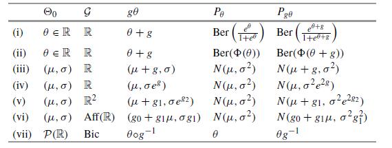
A modification of the preceding model retains the mean vectors, while the covariance matrix is unrestricted but constant over units. Find an expression for the maximum-likelihood estimate of the treatment effect. g G 0 ER R o (i) (ii) (iii) (iv) (, o) R (v) (, ) R Aff(R) (vi) (u, o) (vii) P(R) Bic
Show that the treatment effect in both preceding exercises is a group action on Gaussian distributions. What is the group, and how does it act? In only one case is the action on distributions induced by an action on the sample space. Explain.
Let \(\Theta_{0}=(0,1)\) and let \(P_{\theta}\) be the iid Bernoulli model \(\operatorname{Ber}(\theta)\). Let \(\mathcal{G}\) be the additive group of addition modulo one, so that \(P_{g \theta}=\operatorname{Ber}(\theta+g)\) is the Bernoulli model with parameter \(\theta+g\) modulo one. Explain
By writing the complex vector \(z\) and the Hermitian matrix \(\Gamma\) as a linear combination of real and imaginary parts, show that the Hermitian quadratic form \(z^{*} \Gamma z\) reduces to the following linear combination of real quadratic forms:\(\left(x^{\prime}-i y^{\prime}ight)
Show that the maximum-likelihood estimate of \(\beta\) satisfies\[\left[X^{\prime} K^{\prime}\left(K V K^{\prime}ight)^{-1} K Xight] \hat{\beta}=X^{\prime} K^{\prime}\left(K V K^{\prime}ight)^{-1} Z=X^{\prime} W Q Y\]where \(Q: \mathcal{H} ightarrow \mathcal{H}\) is the orthogonal projection with
Deduce that the composite linear transformation \(Y \mapsto L_{1} Y=Q \hat{\mu}\) is also a projection, and that it is the orthogonal projection whose image is the \(p\)-dimensional subspace \(Q \mathcal{X}\).
Show that the zero-mean exchangeable Gaussian process in Sect. 15.3.3 with covariances\[\operatorname{cov}\left(Y_{r}, Y_{s}ight)=\sigma_{0}^{2} \delta_{r s}+\sigma_{1}^{2}\]has a dynamic or sequential representation beginning with \(Y_{0}=0\) followed by\[Y_{n+1}=\frac{n \theta \bar{Y}_{n}}{1+n
For fixed \(v>0\), show that the Matérn measures are mutually consistent in the sense that \(M_{d+1}(A \times \mathbb{R})=M_{d}(A)\) for all \(d \geq 0\) and subsets \(A \subset \mathbb{R}^{d}\). In other words, show that \(M_{d}\) is the marginal distribution of \(M_{d+1}\) after integrating out
Consistency and finiteness together imply that the normalized Matérn measures define a real-valued process \(X_{1}, X_{2}, \ldots\) in which \(M_{n} / \Gamma(v)\) is the joint distribution of the finite sequence \(X[n]=\left(X_{1}, \ldots, X_{n}ight)\). This process-a special case of the Gosset
For the Matérn process, show that the sequence of partial averages \(\bar{X}_{n}\) has a limit \(\bar{X}_{\infty}=\lim _{n ightarrow \infty} \bar{X}_{n}\). For \(n \geq 2\), what can you say about the conditional distribution of \(\bar{X}_{\infty}\) given \(X[n]\) ? Consider separately the cases
One definition of the Bessel-K function is the integral\[\int_{0}^{\infty} \frac{\cos (\omega t) d \omega}{\left(1+\omega^{2}ight)^{v+1 / 2}}=\frac{\sqrt{ } \pi}{2^{v} \Gamma(v+1 / 2)} \times|t|^{v} \mathcal{K}_{v}(t)\]Deduce that \(\mathcal{K}_{v}(\cdot)\) is symmetric and that\[\lim _{t ightarrow
Special Gaussian family on \(\mathbb{C}^{3}\) : Let \(ho=\left(ho_{1}, ho_{2}, ho_{3}ight)\) be a real vector, and let \(Z=\left(Z_{1}, Z_{2}, Z_{3}ight)\) be a zero-mean complex Gaussian variable with covariance matrix of the form\[\operatorname{cov}\left(Z, Z^{*}ight)=\left(\begin{array}{ccc}1 &
If \(Z: \mathbb{R}^{3} ightarrow \mathbb{R}^{3}\) is the Gaussian process with parameter \((\omega, ho)\) as defined in the preceding exercise, and \(R\) is a \(3 \mathrm{D}\) rotation, show that the domain-rotated process \(x \mapsto Z\left(R^{\prime} xight)\) is Gaussian with parameter \((R
Let \(p, q\) be purely imaginary quaternions. Find the matrix representation \(\chi_{4}(p \bar{q})\) of the quaternion product \(p \bar{q}\), and show how this is related to \(\chi(x)\) in (16.25) and \(\chi(u \times v)\) in Sect. 16.7.4.
Let \(\psi_{0}(y)=e^{-y^{2} / 2} / \sqrt{2 \pi}\) be the standard normal density. Assume that \(Y_{1}, \ldots, Y_{n}\) are independent standard normal. Show that the random variables \(X_{i}=\) \(\psi_{1}\left(Y_{i}ight) / \psi_{0}\left(Y_{i}ight)\) have unit mean, and hence, by the law of large
Show that the random variables \(X_{i}=\psi_{1}\left(Y_{i}ight) / \psi_{0}\left(Y_{i}ight)\) in the preceding exercise have a density whose tail behaviour is \(1 / f(x) \sim x^{2} \log (x)^{3 / 2}\) as \(x ightarrow \infty\).
What does the preceding equation imply about the fraction of non-negligible signals among sites in the sample such that \(\left|Y_{i}ight| \geq 3\) ?
Welham and Thompson (1997) discuss two possibilities for a Gaussian likelihood-ratio statistic. For arbitrary mean vector \(\mu\), inner product matrix \(W=\) \(\Sigma^{-1}\), and \(W\)-orthogonal projection \(Q\) with \(\operatorname{kernel} \mathcal{K}=\operatorname{span}(K)\), W\&T define the
For the balanced block design in the preceding exercise, show that the implied distribution for residuals is a two-parameter full exponential-family model with canonical sufficient statistic \(\mathrm{SS}_{W}, \mathrm{SS}_{B}\). Hence deduce that the residual maximumlikelihood estimate
Show that the REML estimate with positivity constraint satisfies \(1+b \hat{\theta}=\) \(\max (F, 1)\). What is the REML estimate for the second component? Express the constrained REML likelihood-ratio statistic as a function of \(F\), and compute the atom at the origin.
To test for equality of variances in \(k\) blocks of sizes \(n_{1}, \ldots, n_{k}\), the REML procedure goes as follows. First, \(\mathrm{bl} k\) is the \(k\)-dimensional subspace of \(\mathbb{R}^{n}\) spanned by the block indicators \(b_{1}, \ldots, b_{k}\). Second, \(I_{r}\) is the restriction of
Let \(Y\) be a non-negative random variable with cumulants \(\kappa_{r}\) such that \(\kappa_{r} / \kappa_{1}^{r}=\) \(O\left(ho^{r-1}ight)\) as \(ho ightarrow 0\). In other words, the scale-free variable \(Z=Y / \kappa_{1}\) has variance \(ho=\kappa_{2} / \kappa_{1}^{2}\), which is the squared
Show that the transformation \(\mathbb{R}^{n} ightarrow \mathbb{R}^{n}\) defined by\[\bar{u} \mapsto \bar{u}+\text { const }, \quad u_{i}-\bar{u} \mapsto \lambda\left(u_{i}-\bar{u}ight)\]is linear and invertible with Jacobian \(J=|\lambda|^{n-1}\). Here, \(\bar{u}\) is the mean of the components of
As a function of \(\lambda\), show that the transformation \(\mathbb{R}_{+}^{n} ightarrow \mathbb{R}^{n}\)\[(g y)_{i}=\frac{y_{i}^{\lambda}-1}{\lambda \dot{y}^{\lambda-1}}\]is continuous at \(\lambda=0\), and that the Jacobian is the absolute value of\[\frac{1}{\lambda}+\frac{\lambda-1}{n \lambda}
Repeat the preceding exercise taking \(\mathcal{X}=\mathbf{1}\), and \(\Sigma\) a linear combination of the block matrices \(I_{n}\), row and col.
In the balanced case with no missing cells, the standard analysis first reduces the data to 24 rat averages \(\bar{Y}_{i .}\), the treatment and control averages \(\bar{Y}_{T}, \bar{Y}_{C}\), and the overall average \(\bar{Y}_{. .}\). The sum of squares for treatment effects is\[\mathrm{SS}_{T}=70
The \(F\)-ratio reported by anova (...) for treatment effects is not the ratio shown above. At least one is misleading for this design. Which one? Explain your reasoning.
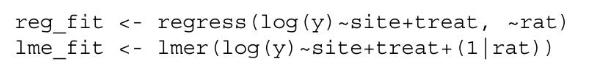
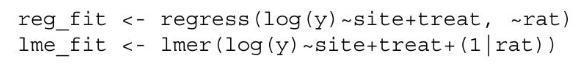
REML, or residual maximum likelihood, is the standard method for the estimation of variance components: see Chap. 18 for details. Both regress () and lmer () allow other options, but both use REML as the default. However, lmer () constrains the coefficients to be positive, whereas regress () allows
A quantitative factor \(x\) with four equally-spaced levels \(0,1,2,3\) may be coded using either the indicator basis \(e_{0}, e_{1}, e_{2}, e_{3}\) (such that \(e_{r}(i)=I\left(x_{i}=right)\) ) or the polynomial basis \(x^{0}, x^{1}, x^{2}, x^{3}\) (with \(x^{0}=1, x^{1}=x\) ). Show that, if every
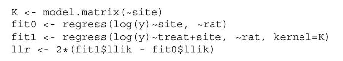
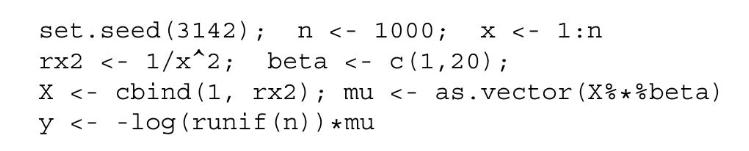
Parameter estimates reported in Sect. 1.5 were computed using the code in Exercise 1.4. Following recommendations in Sect. 18.5, the likelihood ratio statistic for treatment effects was computed using the codeModify this code to obtain the likelihood-ratio statistic for site effects.Data From
It is possible that treatment could have an effect on variances in addition to its effect on the mean. Investigate this possibility by replacing the identity matrix with two diagonal matrices \(D_{0}\) and \(D_{1}\) such that \(D_{0}+D_{1}=I_{n}\), and using some version of the codeReport the two
The set of linear functionals \(\mathbb{R}^{n m} ightarrow \mathbb{R}\) is called the dual vector space; it has dimension \(m n\). Show that the column and row totals \(Y \mapsto Y_{. r}\) and \(Y \mapsto Y_{i \text {. are }}\) linear functionals, and that they are linearly independent. Show that
Use the averages for the six saws A-F\[2.122,2.060,1.975,2.070,2.156,1.920\]to compute the brand sum of squares on two degrees of freedom, the saw replicate sum of squares on three degrees of freedom, and the \(F\)-ratio (ratio of mean squares). Why is this two-part decomposition structurally
In the simple linear model setting, the \(F\)-ratio for testing the hypothesis \(\mu \in \mathcal{X}_{0}\) versus \(\mu \in \mathcal{X}_{1}\) is the ratio of mean squares\[F=\frac{\left\|Q_{0} Yight\|^{2}-\left\|Q_{1} Yight\|^{2}}{\left\|Q_{1} Yight\|^{2}} \frac{n-p_{1}}{p_{1}-p_{0}}\]where
For a Latin-square design of order \(m\), show that the last term in the preceding decomposition can be split into two parts associated with letters. Show also that the five-part decomposition is invariant with respect to permutation of rows, columns and letters.
Hypergeometric simulation in Sect. 3.3.5 implies a symmetric null distribution with standard deviation 0.23 for the weighted sample correlation of homogamic pairs. One suggested alternative to random matching is to generate the null distribution by randomly permuting the vector \(\left(\pi_{2, i},
The advice sometimes given for the validity of the \(\chi^{2}\) approximation to the null distribution of Pearson's statistic is that the minimum expected value should exceed a suitable threshold, usually in the range 3-5. However, the mean count for the birth-death table is 2.42 , so the expected
Check the calculations reported in the penultimate paragraph of Sect. 3.4.2 for Bortkewitsch's horsekick data. Compute the row and column totals, and simulate the null distribution of X2X2 by random matching. Superimpose the χ2247χ2472 density on a histogram of the simulated values. Find two
Explain where the factor \(1-r\) comes from in the penultimate paragraph of Sect. 3.3.5.
Bearing in mind that the heights are measured to the nearest millimetre, comment briefly on the magnitude of the estimated variance components for the FBM model.
In Table S2 of their Appendix, Villa et al. fit the eight-dimensional factorial model host:sex:time to the first principal component values on 3096 lice. Show that this is equivalent to fitting four separate linear regressions \(E\left(Y_{u}ight)=\alpha+\beta t_{u}\), with one intercept and one
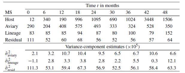
The sex coefficient in Table \(\mathrm{S} 2\) is -2.437 . Which combination of the four \(\alpha\)-values in the previous exercise does this correspond to? MS Host 12 Aviary 290 Lineage 83 Residual 111 8 aviary lineage resid 36 1024 324 80 100 52 56 Variance-component estimates (x10) 2.1 3.2 10.7
The host coefficient in Table S2 is 0.449 with standard error 0.159 . What does this imply about the average or expected baseline values for the four subgroups? MS Host 12 Aviary 290 Lineage 83 Residual 111 8 aviary lineage resid 36 1024 324 80 100 52 56 Variance-component estimates (x10) 2.1 3.2
A variety of other smoothing techniques can be employed to illustrate longterm secular trends. Pick your favourite kernel density smoother, apply it to the temperature series, and compare the fitted curve with the Bayes estimates described above.
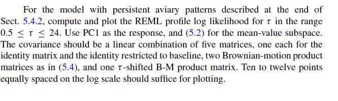
Use the profile log likelihood plot in the previous exercise to obtain a nominal 95\% confidence interval for \(\tau\).Data From previous exercise Section 5.4.2 For the model with persistent aviary patterns described at the end of Sect. 5.4.2, compute and plot the REML profile log likelihood for
Virtual randomization requires the timezero average for feral hosts to be the same as that for giant runts, but the temporal trends are otherwise unconstrained. It appears that the model matrix spanning this subspace is not constructible using factorial model formulae. Explain how to construct the
Use the fitted model from the previous exercise to compute the linear trend coefficient\[\frac{\sum t\left(\hat{\gamma}_{1}(t)-\hat{\gamma}_{0}(t)ight)}{\sum t^{2}}\]and its standard error. You should find both numbers in the range \(0.013-0.015\) per month, similar to, but not exactly the same as
For the non-seasonal frequencies, use \(g \operatorname{lm}()\) to fit the additive exponential model\[E\left(|\hat{Y}(\omega)|^{2}ight)=\beta_{0}+\beta_{1} \exp \left(-|2 \pi \lambda \omega|^{1 / 2}ight)\]for various values of \(\lambda\) in the range \(7-14\) days or \(0.02-0.04\) years. In this
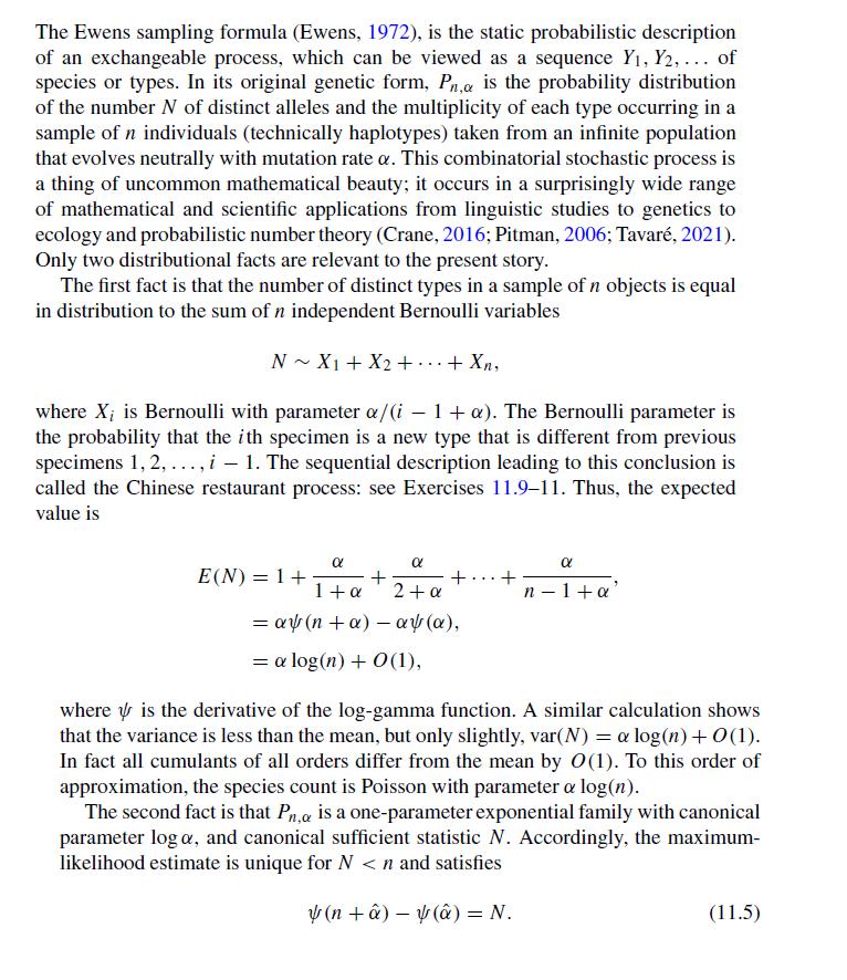
To the order of approximation used in Sect. 11.6, show that the maximumlikelihood estimate, \(\hat{\alpha}\left(T_{n}ight)\), of the species-diversity parameter as a function of the cumulative species count \(T_{n}\), defines a martingale.Data From Section 11.6 The Ewens sampling formula (Ewens,
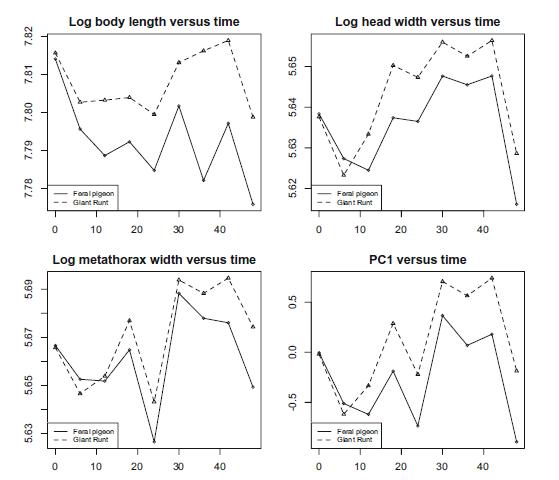
Download the data, compute the averages at each time point for the two pigeon breeds, and reconstruct the plots in Figs. 5.1 and 5.2. 7.82 7.81 7.80 7.79 7.78 5.69 5.67 5.65 5.63 0 Log body length versus time 0 Feralpigaon Giant Runt 10 Feralpigeon Giant Runt 20 Log metathorax width versus time 10
The coefficient of variation is the standard-deviation-to-mean ratio, which is often reported as a percentage. For body length or other size variables, the coefficient of variation is essentially the same as the standard deviation of the logtransformed variable. Compute the coefficient of variation
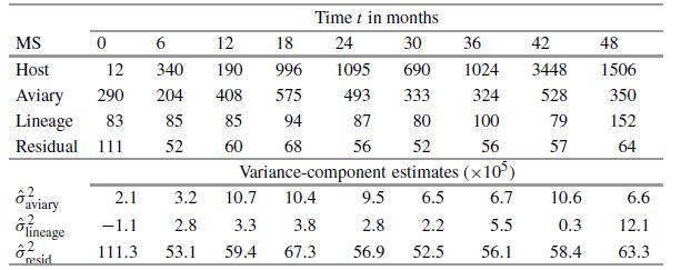
Use anova (. . . ) to re-compute the mean squares in Table 5.2. Use Bartlett's statistic (Exercise 18.9) to test the hypothesis that the residual mean squares have the same expected value at all time points. What assumptions are needed to justify the null distribution? MS 6 12 Host 12 340 190
For the model (5.3), what is the expected value of the within-lineage mean square at time \(t\) ? For the Brownian-motion model (5.4), show that the variance of \(Y_{u}\) increases linearly with time. What is the expected value of the within-lineage mean square?
Use lmer (. . . ) to fit the variance-components model (5.3) to the log body length with (5.2) as the mean-value subspace. Report the two slopes, the slope difference, and the three standard errors.
Compute the four covariance matrices \(V_{0}, \ldots, V_{3}\) that occur in (5.4). Let \(Q\) be the ordinary least-squares projection with kernel (5.2). Compute the four quadratic forms \(Y^{\prime} Q^{\prime} V_{r} Q Y\) and their expected values as a linear function of the four variance
For \(n=100\) points \(t_{1}, \ldots, t_{n}\) equally spaced in the interval \((0,48)\), compute the matrix\[\Sigma_{i j}=\delta_{i j}+\theta\left(t_{i} \wedge t_{j}ight)\]for small values of \(\theta\), say \(0 \leq \theta \leq 0.02\). Find the maximum-likelihood estimate of \(\beta\) in the
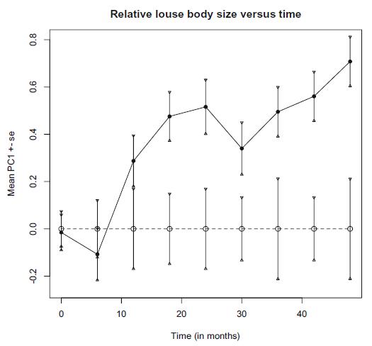
Distributional invariance. Consider a simplified version of the louse model in which there are 16 feral and 16 giant runt pigeons, no sex differences between lice, and no correlations among measurements. Two lice are associated with each bird at baseline, and two at each subsequent time \(t=1,
The model in the previous two exercises has a baseline variance that is larger than the non-baseline residual variance. What is the ratio of fitted variances?
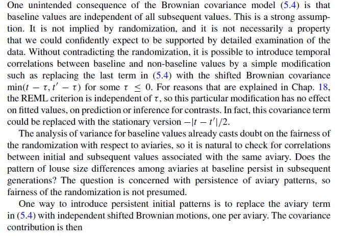
The fact that measured lice were not returned to their hosts is an interference in the system that may reduce or eliminate temporal correlations that would otherwise be expected. One mathematically viable covariance model that is in line with virtual randomization, replaces each occurrence of \(t
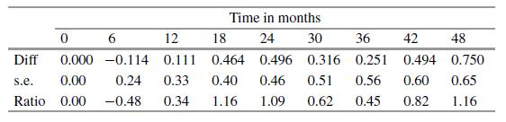
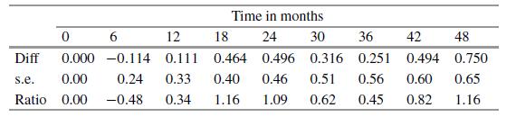
Construct two versions of Table 5.4, one based on the modified block-factor model, and one based on the combined variance model that includes both. Comment on any major discrepancy or difference in conclusions based on the various models. 0 0.000 s.e. 0.00 Ratio 0.00 Diff Time in months 24 6 12 18
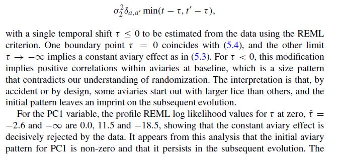
Let \(0
A vector \(x \in \mathbb{R}^{N}\) may be regarded as a function \([N] ightarrow \mathbb{R}\), in which case the composition \(x \varphi\) is a function \([n] ightarrow \mathbb{R}\) or a vector in \(\mathbb{R}^{n}\). Show that Fisher's
The U.K. Met Office maintains a longer record of monthly average and annual average temperatures for Central England from 1659 onwards in the filehttps://www.metoffice.gov.uk/hadobs/hadcet/cetml1659on.datCheck the format, download the data, and plot the annual average temperature as a time series.
The U.K. Met Office site https://www.metoffice.gov.uk/ keeps long-term weather records-temperature, rainfall, and so on-for a range of stations in Great Britain and Northern Ireland. Monthly rainfall totals for Oxford from 1853 onwards are available in the fileCheck the format, download the data,
Let \(\left(\varepsilon_{k}, \varepsilon_{k}^{\prime}ight)_{k \geq 0}\) be independent and identically distributed standard Gaussian variables. For real coefficients \(\sigma_{k}\), show that the random function\[\eta(t)=\sum_{k=0}^{\infty} \sigma_{k} \varepsilon_{k} \cos (k t)+\sigma_{k}
Verify the following trigonometric integral for integer \(k\) :\[\int_{0}^{2 \pi} \sin (x / 2) \cos (k x) d x=\frac{-4}{4 k^{2}-1} .\]Hence find the coefficients \(\lambda_{k}\) in the Fourier expansion of the function\[2 / \pi-\sin (x / 2)=\sum_{k=0}^{\infty} \lambda_{k} \cos (k x)\]for \(0 \leq x
Simulate and plot a random function \(\eta(\cdot)\) on \((0,2 \pi)\) whose covariance is \(\pi / 2-\ell\left(t, t^{\prime}ight)\), where \(\ell(\cdot)\) is the arc-length metric. This function is less well behaved than the chordal function because half of its Fourier coefficients are zero, so the
A real-valued process \(Y(\cdot)\) is called a Gaussian random affine function if the differences \(Y(t)-Y\left(t^{\prime}ight)\) are Gaussian with covariances satisfying\[\operatorname{cov}\left(Y(x)-Y\left(s^{\prime}ight),
Let \(K\) be the covariance function of a stationary process on the real line such that \(K\) is twice differentiable on the diagonal, i.e.,\[K\left(t, t^{\prime}ight)=1-\left(t-t^{\prime}ight)^{2}+o\left(\left|t-t^{\prime}ight|^{2}ight) .\]Suppose that \(Y\) is stationary with covariance
Let \(K\left(t, t^{\prime}ight)=\sigma^{2} \exp \left(-\left|t-t^{\prime}ight| / \lambdaight)\) be the scaled exponential covariance, and let \(Y\) be a zero-mean Gaussian process with covariance \(K\). Show that the longrange limit with \(\sigma^{2} \propto \lambda\) is such that the deviation
Let \(Y_{1}, \ldots, Y_{n}\) be independent and identically distributed standard exponential variables, and let \(0 \leq Y_{(1)} \leq Y_{(2)} \leq \cdots \leq Y_{(n)}\) be the order statistics. Show that \(Y_{(1)} \geq t\) if and only if \(Y_{i} \geq t\) for \(1 \leq i \leq n\), and deduce that \(n
Use fft () to compute the Fourier coefficients for the temperature series on a whole number of years, identify and remove the frequencies that are seasonal, average the power-spectrum values in successive non-overlapping frequency blocks of a suitable size, and plot the log averages against the
Include the inverse-square frequency as an additional covariate in the exponential model for the power spectrum. In principle, this means re-computing \(\hat{\lambda}\). Compute the Wilks statistic, which is the reduction in deviance or twice the increase in log likelihood. Also compute on the Wald
Ordinarily, Wald's likelihood ratio statistic is essentially the same as Wilks's statistic, which in one-parameter problems, is the squared ratio of the estimate to its standard error. But there are exceptional cases where a substantial discrepancy may occur, and variance-components models provide
For \(0
Use the function \(\mathrm{COv}(\mathrm{cbind}(\mathrm{S} 1[\ldots])\) ) to compute the sample covariance matrix of the four phoneme inventory variables. What does this tell you?
Use the function \(q r(\operatorname{cbind}(S 1[\ldots]))\) \$rank to deduce that total phoneme diversity is a linear combination of the three constituents. Find the coefficient vector.
The function vdist \((x 0,1)\) returns a list of linguistic distances from the designated point \(\mathrm{x} 0\) in linguistic region 1 to each of the 504 language locations. Show that Atkinson's distance variable \(\mathrm{S} 1 \$ \mathrm{Dbo}\) implies that his best-fitting origin lies somewhere
Assuming the Out-of-Africa hypothesis, total phoneme inventory necessarily depends not just on distance to the origin but also on the speaker population size. By minimizing the residual sum of squares over continental Africa, find the bestfitting origin under the linearity
Which language has the greatest vowel inventory in the Santoso compilation, and which has the least? Which language has the greatest consonant inventory, and which has the least?
Expand the spreadsheet so that it is indexed by bees rather than by colonies. Check that the two versions of the lmer () code produce the same output for the expanded spreadsheet as they do for the compact format.
Plot the average reproductive score against calendar year. Is the range of annual averages high or low in relation to the reproductive scale \(0-4\) ? Does this plot suggest serial correlation?
Each bird in this study has a sequence length in the range \(0-\mathrm{xx}\). Compute the histogram of sequence lengths. How many sequences are empty? Report the average and the maximum length? What fraction of the birds are one-time breeders?
Show that the model (10.1) implies exchangeability of initial values \(Y_{i, 1} \sim\) \(Y_{j, 1}\) for every pair of birds, whether recorded in the same year or in different years.
What evidence is there in the data suggesting serial correlation in the year effects? Can the fit be improved using a model containing non-trivial serial correlation? Extend the model and report a likelihood-ration statistic.
What evidence is there in the data suggesting serial correlation in the year effects? Can the fit be improved using a model containing non-trivial serial correlation? Extend the model and report a likelihood-ration statistic.
The black-footed ferret is an endangered species; it belongs to the weasel family. A ferret-breeding program has been established by various zoos throughout the United States to study the factors that affect breeding success in captive ferrets. The sample consists of 664 females, 375 males, and
For integer \(n \geq 1\), a partition \(B\) of the set \([n]=\{1, \ldots, n\}\) is a set of disjoint non-empty subsets called blocks whose union is \([n]\). A partition into \(k\) blocks, can be written as \(B=\left\{b_{1}, \ldots, b_{k}ight\}\), with the understanding that \(B\) is a set of
One of the simplest static versions of the Ewens sampling formula is stated as a probability distribution on the set of partitions of the finite set \([n]\) as follows:\[P_{n, \alpha}(B)=\frac{\alpha^{\# B} \prod_{b \in B}(\# b-1) !}{\alpha^{\uparrow n}}\]where \(\alpha^{\uparrow
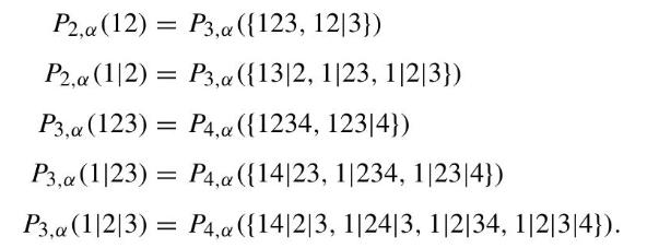
By direct calculation, show that the Ewens distributions satisfy the following conditions:Show that \(P_{4, \alpha}\) is the marginal distribution of \(P_{5, \alpha}\) when the element 5 is removed from the set [5]. Hence calculate the conditional distribution \(P_{5, \alpha}(x \mid B)\) for \(x
Let \(B \sim P_{n, \alpha}\) be the partition after \(n\) customers in the Chinese restaurant process with parameter \(\alpha\), and let \(\hat{\alpha}(B)\) be the maximum-likelihood estimate. One way to approximate the variance of \(\hat{\alpha}(B)\) is to generate bootstrap samples \(B_{1}^{*},
In the non-parametric bootstrap, the configuration \(B\) is regarded as a list of \(n\) tables in order of occupation. Each non-parametric bootstrap sample is a sequence of \(n\) tables drawn with replacement from the empirical distribution of tables. Although \(\hat{\alpha}\left(B^{*}ight) \leq
Each land parcel belongs to the first or inner ring, the second ring, the third ring, or beyond. To be clear, the rings are disjoint, so the phrase 'second ring' excludes the first. A district may straddle two or more rings. What sort of variable is ring?

Showing 4900 - 5000 of 5106

First
38
39
40
41
42
43
44
45
46
47
48
49
50
51
52

Step by Step Answers

Services

Sitemap
Fun
Definitions
Become Tutor
Used Textbooks
Study Help Categories
Recent Questions
Expert Questions
Campus Wear
Sell Your Books

Company Info

Security
Copyrights
Privacy Policy
Terms & Conditions
SolutionInn Fee
Scholarship
Online Quiz
Give Feedback, Get Rewards

Get In Touch

About Us
Contact Us
Career
Jobs
FAQ
Student Discount
Campus Ambassador

Secure Payment

Download Our App

© 2026 SolutionInn. All Rights Reserved