New Semester
Started
Get
50% OFF
Study Help!
--h --m --s
Claim Now
Question Answers
Textbooks
Find textbooks, questions and answers
Oops, something went wrong!
Change your search query and then try again
S
Books
FREE
Study Help
Expert Questions
Accounting
General Management
Mathematics
Finance
Organizational Behaviour
Law
Physics
Operating System
Management Leadership
Sociology
Programming
Marketing
Database
Computer Network
Economics
Textbooks Solutions
Accounting
Managerial Accounting
Management Leadership
Cost Accounting
Statistics
Business Law
Corporate Finance
Finance
Economics
Auditing
Tutors
Online Tutors
Find a Tutor
Hire a Tutor
Become a Tutor
AI Tutor
AI Study Planner
NEW
Sell Books
Search
Search
Sign In
Register
study help
business
categorical data analysis
An Introduction To Categorical Data Analysis 1st Edition Alan Agresti - Solutions
. Refer to the previous problem.a. Calculate the binomial probabilities for N = 2 when the probability of a head for each flip equals (i) = .6, (ii) = .4.b. Suppose we observe Y = 1. Calculate and sketch the likelihood function.c. Using the plotted likelihood function from (b), show that the ML
. In his autobiography A Sort of Life, British author Graham Greene described a period of severe mental depression during which he played Russian Roulette. This "game" consists of putting a bullet in one of the six chambers of a pistol, spinning the chambers to select one at random, and then firing
. A sample of women suffering from dysmenorrhea have been taking an analgesic designed to diminish the effects. A new analgesic is claimed to provide greater relief. After trying the new analgesic, 40 women reported greater relief with the standard analgesic, and 60 reported greater relief with the
. Refer to the previous problem. The researchers wanted a sufficiently large sample to be able to estimate the probability of preferring the new analgesic to within .08, with confidence .95. If the true probability is .75, how large a sample is needed to achieve this accuracy? (Hint: How large
. Newsweek magazine (March 27, 1989) reported results of a poll about religious beliefs, conducted by the Gallup Organization. Of 750 American adults, 24% believed in reincarnation. Treating this as a random sample, construct and interpret a 95% confidence interval for the true proportion of
. A criminologist wants to estimate the proportion of U.S. citizens who live in a home in which firearms are available. The 1991 General Social Survey asked respondents, "Do you have in your home any guns or revolvers?" Of the respondents, 393 answered "yes" and 583 answered "no." Construct a 90%
. If Y is a variate and c is a positive constant, then the standard deviation of the distribution of cY equals co (Y). Suppose Y is a binomial variate, and let p = Y/N. Show that (p)=(1-T)/N. Explain why it is easier to get a close estimate of when it is near 0 or 1 than when it is near.
. A variate has a Poisson distribution, with unknown parameter . The sole observation equals 0.a. Find and plot the likelihood function over the space of potential values for .b. What is the ML estimate of ? (Recall: The ML estimate of equals the sample mean.)
. Using calculus, it is easier to derive the maximum of the log of the likelihood function, L = log 1, than the likelihood function / itself. Both functions have maximum at the same value, so it is sufficient to do either.a. Calculate the log likelihood L() for the binomial distribution (1.2.2).b.
. Show that a value o for which the statistic z = (p- To)/(1-T)/N takes some fixed value zo is a solution to the equation (1 + 2/N) m +(-2p- /N)To+p = 0. Hence, using the formula x = (-b b2-4ac)/2a for solving the quadratic equation ax + bx + c = 0, obtain the limits for the 95% confidence interval
A Swedish study considered the effect of low-dose aspirin on reducing the risk of stroke and heart attacks among people who have already suffered a stroke (Lancet 338: 1345-1349 (1991)). Of 1360 patients, 676 were randomly assigned to the aspirin treatment (one low-dose tablet a day) and 684 to a
In the United States, the estimated annual probability that a woman over the age of 35 dies of lung cancer equals .001304 for current smokers and .000121 for nonsmokers (M. Pagano and K. Gauvreau, Principles of Biostatistics, Belmont, CA: Duxbury Press, 1993, p. 134).a. Calculate and interpret the
The odds ratio between treatment (A, B) and response (death, survival) equals 2.0.a. Explain what is wrong with the interpretation, "The probability of death with treatment A is twice that with treatment B." Give the correct interpretation.b. When is the quoted interpretation in (a) correct, in an
An estimated odds ratio for adult females between the presence of squamous cell carcinoma (yes, no) and smoking behavior (smoker, non-smoker) equals 11.7 when the smoker category consists of subjects whose smoking levels is 0 < < 20 cigarettes per day; it is 26.1 for smokers with s 20 cigarettes
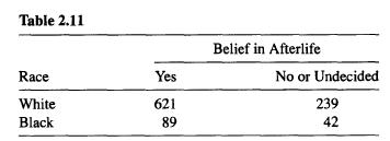
Table 2.11 was taken from the 1991 General Social Survey.a. Identify each classification as a response or explanatory variable.b. Describe the association. Interpret the direction and strength of association.c. Obtain a 95% confidence interval for a population measure, and interpret. Table 2.11
A poll by Louis Harris and Associates of 1249 adult Americans in July 1994 indicated that 36% believe in ghosts and 37% believe in astrology. Can we compare the proportions using inferential methods for independent binomial samples? Explain.
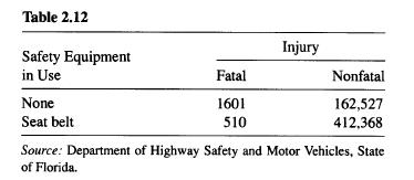
Table 2.12 is based on records of accidents in 1988 compiled by the Department of Highway Safety and Motor Vehicles in Florida. Compute and interpret the sample odds ratio, relative risk, and difference of proportions, and explain why the odds ratio approximately equals the relative risk. Table
In an article about crime in the United States, Newsweek magazine (Jan. 10, 1994) quoted FBI statistics stating that of all blacks slain in 1992, 94% were slain by blacks, and of all whites slain in 1992, 83% were slain by whites. Let Y denote race of victim and X denote race of murderer.a. Which
A 20-year study of British male physicians (R. Doll and R. Peto, British Med. J., 2: 1525-1536 (1976)) noted that the proportion who died from lung cancer was .00140 per year for cigarette smokers and .00010 per year for nonsmokers. The proportion who died from heart disease was .00669 for smokers
Refer to Table 2.1.a. Construct a 90% confidence interval for the difference of proportions, and interpret.b. Construct a 90% confidence interval for the odds ratio, and interpret.c. Conduct a test of statistical independence. Interpret.
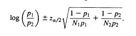
A large-sample confidence interval for the log of the relative risk isAntilogs of the endpoints yield an interval for the true relative risk. For Table 2.1, construct a 90% confidence interval. log 1-P Nipi 1-P2 + N2P2
Refer to Table 2.3. Find the P-value for testing that the incidence of heart attacks is independent of aspirin intake, (a) using X2, (b) using G. Interpret results.
Refer to Table 2.4. Do these data provide evidence of an association between myocardial infarction and smoking? Use an inferential procedure, and interpret.
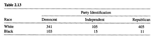
Table 2.13 was taken from the 1991 General Social Survey.a. Test the hypothesis of independence between party identification and race. Interpret.b. Use adjusted residuals to describe the evidence.c. Partition chi-squared into two components, and use the components to describe the evidence. Table
A recent article (D. J. Moritz and W. A. Satariano, J. Clin. Epidemiol., 46: 443-454 (1993)) investigated the relationship between stage of breast cancer at diagnosis (local or advanced) and a woman's living arrangement. Of 144 women living alone, 41.0% had an advanced case; of 209 living with
Give examples of contingency tables for which a chi-squared test of inde- pendence using X or G should not be used, because of (a) sample size, (b) measurement scale.
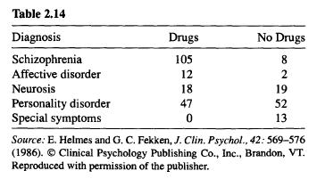
Table 2.14 classifies a sample of psychiatric patients by their diagnosis and by whether their treatment prescribed drugs.a. Report the P-value for a test of independence, and interpret the result.b. Calculate adjusted residuals, and interpret.c. Partition chi-squared into three components to
Refer to Table 7.5 (Chapter 7). Combine data for the two genders, yielding a single 4 X 4 table.a. Use X and G to test independence. Interpret.b. Partition G into three components for three 2 4 tables by (i) comparing the first two income levels on job satisfaction, (ii) comparing the last two
A study on educational aspirations of high school students (S. Crysdale, Int. J. Compar. Sociol., 16: 19-36 (1975)) measured aspirations using the scale (some high school, high school graduate, some college, college grad- uate). For students whose family income was low, the counts in these cate-
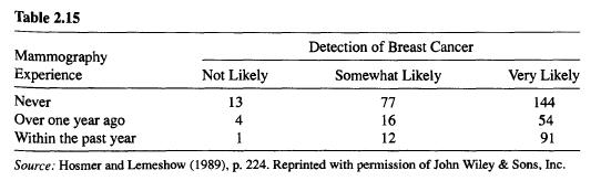
Table 2.15 refers to a study that assessed factors associated with women's attitudes toward mammography (Hosmer and Lemeshow, 1989, p. 220). The columns refer to their response to the question, "How likely is it that a mam- mogram could find a new case of breast cancer?" Analyze these data. Table
Refer to Table 8.12 (Chapter 8). Analyze these data using the methods of this chapter.
A study (B. Kristensen et al., J. Intern. Med., 232: 237-245 (1992)) con- sidered the effect of prednisolone on severe hypercalcaemia in women with metastatic breast cancer. Of 30 patients, 15 were randomly selected to re- ceive prednisolone, and the other 15 formed a control group. Seven of the 15
Refer to the previous problem. Compute the sample odds ratio. Using software, obtain a 95% "exact" confidence interval for the true odds ratio. Interpret, and note the effect of the zero cell count.
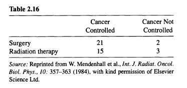
Table 2.16 contains results of a study comparing radiation therapy with surgery in treating cancer of the larynx. Use Fisher's exact test to test Ho: 0 = 1 against Ha: 0 > 1. Interpret results. Table 2.16 Surgery Radiation therapy Cancer Controlled Cancer Not Controlled 21 2 15 3 Source:
Refer to the previous problem.a. Obtain and interpret the one-sided mid-P value. Give advantages and dis- advantages of this type of P-value compared to the ordinary one.b. Obtain and interpret a two-sided exact P-value.
Suppose a researcher routinely conducts tests using a nominal probability of Type I error of .05, rejecting Ho if the P-value satisfies P < .05. Suppose an exact test using X2 has null distribution P(X2 = 0) = .30, P(X = 3) = .62, and P(X29) .08.a. Show that, with the usual P-value, the actual
Refer to Table 2.8.a. Construct the null distributions of the ordinary P-value and the mid P-value, for the one-sided alternative. Compute and compare their expected values.b. Repeat (a) for the test using X for the two-sided alternative.
Consider the 3 3 table having entries, by row, of (4,2,0/2,2,2/0,2,4).a. Using software, conduct an exact test of independence, using X. Interpret.b. Suppose the row and column classifications are ordinal. Using equally- spaced scores, conduct an ordinal exact test. Explain why results differ so
A diagnostic test is designed to detect whether subjects have a certain disease. A positive test outcome predicts that a subject has the disease. Given that the subject has the disease, the probability the diagnostic test is positive is called the sensitivity. Given that the subject does not have
For tests of independence, {j= n;+n+/n}. Show that {ij} have the same row and column totals as the observed data. For 2 x 2 tables, show that their odds ratio equals 1.0. Hence, they satisfy the null hypothesis. (For I XJ tables, the odds ratio equals 1.0 for every 2 2 subtable formed using a pair
The Pearson residual for a cell in a two-way table equals ej (niji).a. Show that they provide a decomposition of the Pearson chi-squared statistic, through X =b. Show that Pearson residuals are smaller than adjusted residuals and thus have smaller variance than standard normal variates.c. For 2 x 2
Formula (2.4.3) has alternative expression X = n(Pij - Pi+P+1)/Pi+P+j For a particular set of {pij), X2 is directly proportional to n. Hence, X can be large when n is large, regardless of whether the association is practically important. Explain why chi-squared tests, like other tests, simply
Let Z denote a standard normal variate. Then Z has a chi-squared distribution with df 1. A chi-squared variate with degrees of freedom equal to df has representation Z++Z, where Z.....Zaf are independent standard normal variates. Using this, show that if Y, and Y2 are independent chi-squared
In murder trials in 20 Florida counties during 1976 and 1977, the death penalty was given in 19 out of 151 cases in which a white killed a white, in 0 out of 9 cases in which a white killed a black, in 11 out of 63 cases in which a black killed a white, and in 6 out of 103 cases in which a black
For all trials in Florida involving homicides between 1976 and 1987, M. Radelet and G. Pierce (Florida Law Review, 43: 1-34 (1991)) reported the following results: The death penalty was given in 227 out of 4645 cases in which a white killed a white, in 92 out of 731 cases in which a black killed a
Smith and Jones are 1 seball players. Smith had a higher batting average than Jones in 1994 and 19 . Is it possible that for the combined data for these two years, Jones had the higher batting average? Explain, and illustrate using data.
Give a "real world" example of three variables X, Y, and Z, for which you expect X and Y to be marginally associated but conditionally independent, controlling for Z.
Based on 1987 murder rates in the United States, the Associated Press reported that the probability a newborn child has of eventually being a murder victim is 0.0263 for nonwhite males, 0.0049 for white males, 0.0072 for nonwhite females, and 0.0023 for white females.a. Find the conditional odds
Using graphs or tables to illustrate, explain what is meant by "no interaction" in modeling a response Y and explanatory variables X and Z, when (a) all variables are continuous (multiple regression), (b) Y and X are continuous, Z is categorical (analysis of covariance), (c) Y is continuous, X and
For three-way contingency tables, when any pair of variables is conditionally independent, explain why there is homogenous association. When there is not homogeneous association, explain why no pair of variables can be conditionally independent.
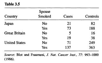
Table 3.5 refers to the effect of passive smoking on lung cancer. It summarizes results of case-control studies from three countries among nonsmoking women married to smokers. Test the hypothesis that having lung cancer is independent of passive smoking, controlling for country. Report the P-value,
Refer to the previous problem. Assume that the true odds ratio between passive smoking and lung cancer is the same for each study. Estimate its value, and use software to find a 95% confidence interval. Interpret. Analyze whether the odds ratios truly are identical.
Table 3.6 shows results of a three-center clinical trial designed to compare a drug to placebo for treating severe migraine headaches. At each center, subjects were randomly assigned to treatments.a. Describe the associations in the partial tables. Are results similar among centers?b. Find the
Refer to Table 3.1. Treating this as a sample, analyze the data.
Refer to Problem 3.2. Test whether the odds ratios are the same at each level of victims' race. Interpret.
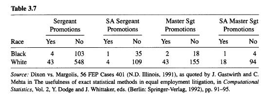
Refer to Table 3.7, which classifies police officers by rank, race, and promotion decisions made in 1988.a. Conduct an exact test of conditional independence of promotion and race, given rank. Interpret, and compare results to the large-sample test.b. Conduct an exact test of whether the odds ratio
Refer to Problem 3.10.a. Use an exact test to conduct this analysis. Compare results to the large- sample test.b. Conduct an exact test that the odds ratio is identical for all three centers. Compare results to the large-sample test.c. Construct and interpret a confidence interval for an assumed
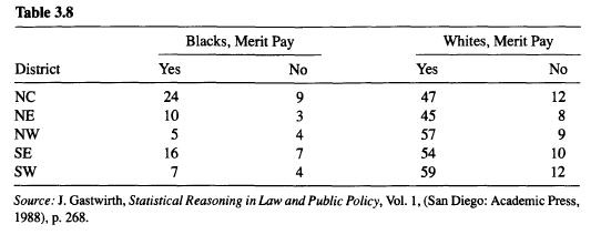
Table 3.8 refers to ratings of agricultural extension agents in North Carolina. In each of five districts, agents were classified by their race and by whether they qualified for a merit pay increase. Analyze these data. Table 3.8 District Yes NC NE NW SE SW 20367 24 10 5 16 Blacks, Merit Pay
Describe the purpose of the link function of a GLM. Define the identity link, and explain why it is not often used with binomial or Poisson data.
Refer to Table 4.1. Refit the linear probability model or the logistic regression model using the scores (i) (0, 2, 4, 6), (ii) (0, 1, 2, 3), (iii). (1, 2, 3, 4). Compare the model parameter estimates under the three choices. Compare the fitted values. What can you conclude about the effect of
Refer to Table 4.2. Let Y = 1 if a crab has at least one satellite, and Y = 0 otherwise. Using weight as the predictor, fit the linear probability model.a. Use ordinary least squares. Interpret the parameter estimates. Find the pre- dicted probability at the highest observed weight of 5.20 kg.
Refer to Table 2.7 on alcohol consumption and infant malformation.a. Using scores {0, .5, 1.5, 4, 7}, fit a linear probability model. Interpret, and compare the sample proportions to the fitted probabilities.b. Fit a logit or probit model, and interpret.
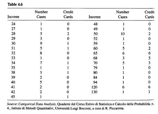
Table 4.6 refers to a sample of subjects randomly selected for an Italian study on the relation between income and whether one possesses a travel credit card (such as American Express or Diners Club). At each level of annual income in millions of lira, the table indicates the number of subjects
An experiment analyzes imperfection rates for two processes used to fabricate silicon wafers for computer chips. For treatment A applied to 10 wafers, the numbers of imperfections are 8, 7, 6, 6, 3, 4, 7, 2, 3, 4. Treatment B applied to 10 wafers has 9, 9, 8, 14, 8, 13, 11, 5, 7, 6 imperfections.
Refer to the previous problem. Conduct the test of Ho A = B by using the fact that if X is Poisson with mean and Y is an independent Poisson variate with mean 2, then X given X + Y is binomial with index n = X + Y and parameter =/( + 2). (Hint: Let X and Y be the total numbers of imperfections for
Refer to Problem 4.6. The wafers are also classified by thickness of silicon coating (z 0, low; z = 1, high). The first five imperfection counts reported for each treatment refer to z = 0 and the last five refer to z = 1. Analyze these data.
Refer to Table 4.2.a. Using weight as the predictor and the number of satellites as the response, fit a Poisson loglinear model. Estimate the mean number of satellites for female crabs of average weight, 2.44 kg.b. Use to describe the effect of weight. Construct a confidence interval for the
Refer to the previous problem.a. Test goodness of fit by grouping levels of weight. Use residuals to describe lack of fit.b. Is there evidence of overdispersion? If necessary, adjust the standard errors for the parameter estimates, and interpret.
Refer to Table 4.2.a. Fit a Poisson loglinear model using both weight and color to predict the number of satellites. Assigning dummy variables, treat color as a nominal factor. Interpret the parameter estimates.b. Estimate the mean number of satellites for female crabs of average weight (2.44 kg)
In Section 4.3.2, refer to the Poisson regression model with identity link for the crab data. Explain why the fit differs from the least squares fit. (Hint: The least squares fit is the same as the ML fit of the GLM assuming normal rather than Poisson random component. What do the two approaches
Refer to the injurious accident data in Section 4.3.4.a. Test the hypothesis of equal rates for men and women using a likelihood- ratio test. Compare results to the Wald test.b. White drivers had 348 injurious accidents in 29.4 thousand years of driving, and black drivers had 147 injurious
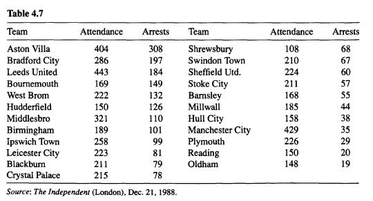
Table 4.7 lists total attendance (in thousands) and the total number of arrests, in the 1987-1988 season for soccer teams in the Second Division of the British football league. (Thanks to Dr. P. M. E. Altham for showing me these data.)a. Let Y denote the number of arrests for a team with total
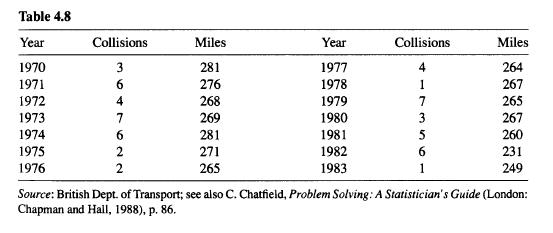
Table 4.8 shows the number of train miles (in millions) and the number of collisions involving British Rail passenger trains between 1970 and 1984. Is it plausible that the collision counts are independent Poisson variates with constant rate over the 14-year period? Respond by testing the goodness
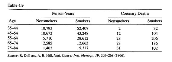
Table 4.9, based on a study with British doctors conducted by R. Doll and A. B. Hill, was analyzed by N. R. Breslow in A Celebration of Statistics, A. C. Atkinson and S. E. Fienberg, eds. (Berlin: Springer-Verlag, 1985).a. For each age, compute the sample coronary death rates per 1000 person-
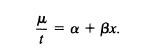
For rate data, the Poisson GLM with identity link isa. Since the model has form at +tx, argue that it is equivalent to a Poisson GLM for the response totals at the various levels of x, using identity link with t and tx as explanatory variables and no intercept or offset terms.b. Fit this model to
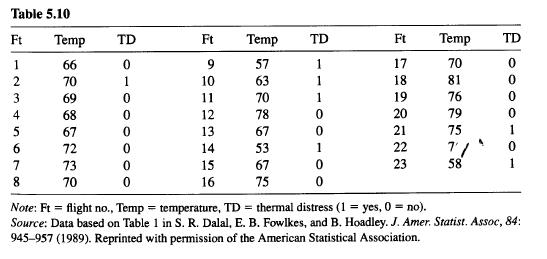
For the 23 space shuttle flights that occurred before the Challenger mission disaster in 1986, Table 5.10 shows the temperature (F) at the time of the flight and whether at least one primary O-ring suffered thermal distress.a. Use logistic regression to model the effect of temperature on the
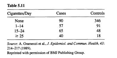
Table 5.11 contains results of a case-control study on the relationship between smoking and myocardial infarction (MI). The sample consisted of young and middle-aged women admitted to 30 coronary units in northern Italy and controls admitted to the same hospitals with other acute disorders. The
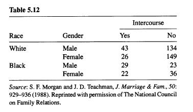
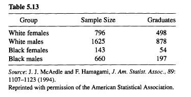
Table 5.12 appeared in a national study of 15 and 16 year-old adolescents. The event of interest is ever having sexual intercourse. Analyze these data, including description and inference about the effects of gender and race, goodness-of-fit and residual analyses, and summary interpretations. Table
According to the Independent newspaper (London, March 8, 1994), the Metropolitan Police in London reported 30,475 people as missing in the year ending March 1993. For those of age 13 or less, 33 of 3271 missing males and 38 of 2486 missing females were still missing a year later. For ages 14-18,
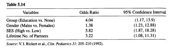
In a study designed to evaluate whether an educational program makes sexually active adolescents more likely to obtain condoms, adolescents were randomly assigned to two experimental groups. The educational program, involving a lecture and videotape about transmission of the HIV virus, was provided
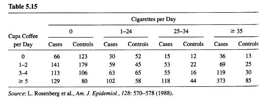
Table 5.15 refers to results of a case-control study about effects of cigarette smoking and coffee drinking on myocardial infarction (MI) for a sample of men under 55 years of age.a. Fit a logit model, treating coffee drinking and cigarette smoking as quali- tative factors. Interpret effects, and
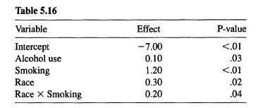
Table 5.16 shows estimated effects for a fitted logistic regression model with squamous cell esophageal cancer (Y = 1, yes; Y = 0, no) as the response variable. Smoking status (S) equals 1 for at least one pack per day and 0 otherwise, alcohol consumption (A) equals the average number of alcoholic
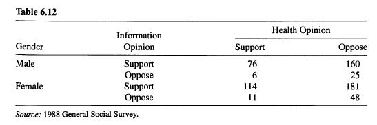
In the 1988 General Social Survey respondents were asked "Do you support or oppose the following measures to deal with AIDS? (1) Have the government pay all of the health care costs of AIDS patients; (2) Develop a government information program to promote safe sex practices, such as the use of con-
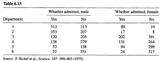
Table 6.13 refers to applicants to graduate school at the University of California at Berkeley for the fall 1973 session. Admissions decisions are presented by gender of applicant, for the six largest graduate departments. Denote the three variables by A = whether admitted, G gender, and D =
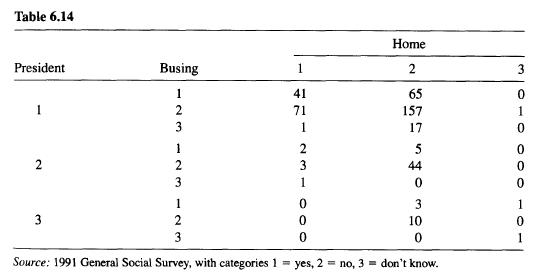
Table 6.14 is from the 1991 General Social Survey. White subjects in the sample were asked: (B) Do you favor busing of (Negro/Black) and white school children from one school district to another?, (P) If your party nominated a (Negro/Black) for President, would you vote for him if he were qualified
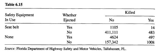
Table 6.15 is based on automobile accident records in 1988, supplied by the state of Florida Department of Highway Safety and Motor Vehicles. Subjects were classified by whether they were wearing a seat belt, whether ejected, and whether killed.a. Find a loglinear model that describes the data
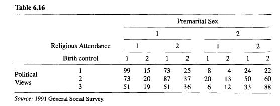
Table 6.16, based on the 1991 General Social Survey, relates responses on four variables: How often you attend religious services (R = At most a few times a year, At least several times a year); Political views (P = Liberal, Moderate,Conservative); Methods of birth control should be available to
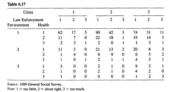
Table 6.17 is taken from the 1989 General Social Survey. Subjects were asked their opinions regarding government spending on the environment (E), health (H), assistance to big cities (C), and law enforcement (L). The common re- sponse scale was (too little, about right, too much). (Note that,
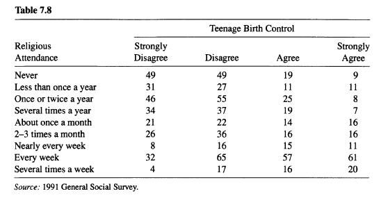
Table 7.8 is taken from the 1991 General Social Survey. Subjects were asked whether methods of birth control should be available to teenagers between the ages of 14 and 16, and how often they attend religious services.a. Fit the independence model, and use residuals to describe lack of fit.b. Using
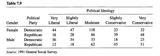
Table 7.9, taken from the 1991 General Social Survey, shows the relation between political party affiliation and political ideology, stratified by gender. Analyze these data. Table 7.9 Political Ideology Political Very Slightly Gender Party Liberal Liberal Moderate Slightly Conservative Very
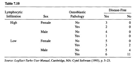
Consider Table 7.10, from a study of nonmetastatic osteosarcoma described in A. M. Goorin, J. Clinical Oncology, 5: 1178-1184 (1987) and the LogXact Turbo User Manual (1993, p. 5-22). The response is whether the subject achieved a three-year disease-free interval.a. Show that each predictor has a
Refer to Problem 6.12 with Table 6.16 and the loglinear model you selected for those data. Draw the association graph for the model. Remark on conditional independence patterns. For each pair of variables, indicate whether the fitted marginal and partial associations are identical.
A GLM has form g(u) = X, for a monotone function g. Explain what each symbol in this formula represents for fitting the ordinary linear regression model to n observations on a normally distributed response and a single predictor.
For Table 6.3, show the matrix representation of loglinear model (AC, AM, CM). Specify the parameter constraints used in your model ma- trix. Show the matrix representation of the corresponding logit model, when M is a response.
Refer to formula (7.5.3) applied to the independence model for a 2 2 table. Show that for the constraints A == 0, for which B = (A, A, ), X has rows (1,0,0), (1,0, 1), (1, 1, 0), (1, 1, 1).
Refer to {ijk = ni+kn+jk/n++k} for model (XZ, YZ). Show that these fitted values have the same X-Z and Y-Z marginal totals as the observed data. For 2 2 K tables, show that Oxy(k) = 1. Illustrate these results for the fit of model (AM, CM) to Table 6.3.
For the model logit(T) = a +x, let (x, y) denote the x and y values for subject i, i = 1,..., N. Suppose y = 0 for all x below some point and y; = 1 for all x above that point. Explain intuitively why B =c. (Note: In technical terms, the sufficient statistics are y, for a and xy; for . For a given
Suppose that all row and column marginal totals of a two-way table are positive, but some cells are empty. Show that all fitted values for the loglinear model of independence (6.1.1) are positive.
Show that a single cell containing any positive count makes a large contribution to X if the fitted value is close to 0. To illustrate, calculate the contribution of (a) a count of 1 in a cell having a fitted value of .01, (b) the count of 2 in the cell having a fitted value of 0.24 for model (AM,
Provide an example of contingency tables in which certain cells contain (a) structural zeroes, (b) sampling zeroes.
Showing 900 - 1000
of 1340
1
2
3
4
5
6
7
8
9
10
11
12
13
14
Step by Step Answers