New Semester
Started
Get
50% OFF
Study Help!
--h --m --s
Claim Now
Question Answers
Textbooks
Find textbooks, questions and answers
Oops, something went wrong!
Change your search query and then try again
S
Books
FREE
Study Help
Expert Questions
Accounting
General Management
Mathematics
Finance
Organizational Behaviour
Law
Physics
Operating System
Management Leadership
Sociology
Programming
Marketing
Database
Computer Network
Economics
Textbooks Solutions
Accounting
Managerial Accounting
Management Leadership
Cost Accounting
Statistics
Business Law
Corporate Finance
Finance
Economics
Auditing
Tutors
Online Tutors
Find a Tutor
Hire a Tutor
Become a Tutor
AI Tutor
AI Study Planner
NEW
Sell Books
Search
Search
Sign In
Register
study help
business
nonparametric statistical inference
An Introduction To Multivariate Statistical Analysis 3rd Edition Theodore W. Anderson - Solutions
5.4. (Sec. 5.2.2) Use Problems 5.2 and 5.3 to show that [T 2/(N - 1)][(N - p)/p]has the Fp. N_p-distribution (under the null hypothesis). [Note: This is the analysis that corresponds to Hotelling's geometric proof (1931).)
5.3. (Sec. 5.2 2) Letwhere U \> ••. , II N are N numbers and x\> ... , X N are independent, each with the distribution N(O, l:). Prove that the distribution of R2/O - R2) is independent of U I, ... , UN' [Hint: There is an orthogonal N X N matrix C that carries (Ill"'" LIN) into a vector
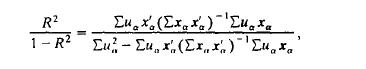
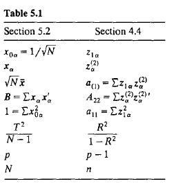
5.2. (Sec. 5.2.2) Show that r2 /(N - 1) can be written as R2/O - R2) with the correspondences given in Table 5.1. Table 5.1 Section 5.2 Section 4.4 X0a - 1/N Zla (2) Za I a Nx B =xx 1-xa T N-1 P N = (2) Azz = z(2)(2) a11 - Cz R 1-R p-1 n
5.1. (Sec. 5.2) Let x" be distributed according to N(". + \3(z" - z), l;), ex =1, ... , N, where z = (1/N)Ez". Let b =[l/Hz" -z)2]ExQ (za -Z),(N - 2)S =E[x,,-i-b(za-z)][xa-i-b(za-Z)l'. and r 1 =Hza -Z)2b'S-lb. Show that T2 has the T2-distribution with N - 2 degrees of freedom. [Hinr: See Problem
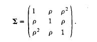
4.49. Suppose X is distributed according to N(O, l:), whereShow that on the basis of one observation, x' = (Xl' x 2• X 3 ). we can obtain a confidence interval for p (with confidence coefficient 1 -a) by using as endpoints of the interval the solutions in I ofwhere xi(a) is the significance point
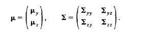
4.48. Missing observations. Let X = (Y' Z')', where Y has p components and Z has q components, be distributed according to N(Il-, l:), whereLet M observations be made on X, and N - M additional observations be made on Y. Find the maximum likelihood estimates of Il- and l:. [Anderson (1957).][Hint:
4.47. (Sec. 4.3) Using the results in Problems 4.43-4.46, prove that the test for PI2.3 ....• p = 0 is equivalent to the usual I-test for 1'2 = O.
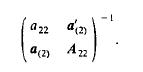
4.46. (Sec. 4.3) Prove that 1/a22.3 .. .. 1' is the element in the upper left-hand corner of -L 022 a (2) a(2) A 22
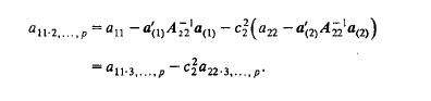
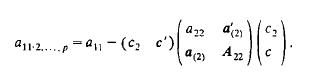
4.45. (Sec. 4.3) In the notation of Problem 4.44, proveHint: Use = a11-2.pa-(1) a (1) - c (an - (2) A'a (2) a11-3p-ca22-3.p
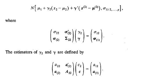
4.44. (Sec. 4.3) Let X' = (Xl' X2 , X(2)') have the distribution MII-,:n The conditional distribution of XI given X 2 = x2 and X(2) = X(2) isShow C2 = a12 .3, . . , pla22 .3, ... ,p. [Hint: Solve for c in terms of c2 and the a's, and substitute.) where N[ 141 + 2 ( x 2 2 ) + ' ( x (2) - l (2)),
4.43. (Sec. 4.3) Prove that if Pij-q+I, ... ,p=O, then ..;N-2-(p-q)rij.q+I ..... pl';1 - r;}.q+ I , ... ,p is distributed according to the t-distribution withN - 2 - (p - q)degrees of freedom.
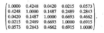
4.42. Let the components of X correspond to scores on tests in arithmetic speed(XI)' arithmetic power (X2 ), memory for words (X3 ), memory for meaningful symbols (X.1), and memory for meaningless symbols (X;). The observed correlations in a sample of 140 are [Kelley (1928»)(a) Find the partial
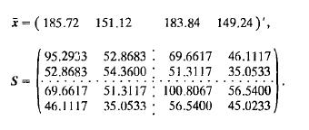
4.41. The estimates of .... and l: in Problem 3.1 are(a) Find the estimates of the parameters of the conditional distribution of (X3,X 4) given (xl,xz); that is, find SZISIII and S22'1 =S2Z -SZISI;ISIZ'(b) Find the partial correlation r~4'12'(e) Use Fisher's Z to find a confidence interval for
4.40. (Sec. 4.4) Prove that (47) is the unique unbiased estimator of R2 based on R2.
4.39. (Sec. 4.4) Prove that (30) is the uniformly most powerful test of R = 0 based on r. [Hint: Use the Neyman-Pearson fundamentallemma.l
4.38. (Sec. 4.4) Show that thl: density of rZ derived from (38) of Section 4.2 is identical with (42) in Section 4.4 for p = 2. [Hint: Use the duplication formula for the gamma function.l
4.37. (Sec. 4.4) Find the distribution of RZ /0 - RZ) by multiplying the density of Problem 4.35 by the dcnsity of all and intcgrating with respect to all'
4.36. (Sec. 4.4) Prove that the noncentrality parameter in the distribution in Problem 4.35 is (all/O"II)lF/(l-IF).
4.35. (Sec. 4.4) Prove that conditional on ZI" = ZI,,' a = 1, ... , n, RZ /0 - RZ) is distributed like T 2/(N* - 1), where T Z = N* i' S-I i based on N* = n observations on a vector X with p* = p - 1 components, with mean vector (c / 0"11)0"(1)(nc z = EZT,,) and covariance matrix l:ZZ'1 = l:zz
4.34. (Sec. 4.4) Invariance of the sample multiple correlation coefficient. Prove that R is a fUllction of the sufficient statistics i and S that is invariant under changes of location and scale of x I a and nonsingular linear transformations of x~2) (that is. xi" = ex I" +d, x~~)* = CX~2) +d, a =
4.33. (See. 4.3) II/variance of Ihe sample partial correiatioll coefficient. Prove that rlc .3 ..... p is invariant under the transformations x;a = aixia + b;x~) + ci' ai> 0, t' = 1, 2, x~')' = Cx~') + b" a = 1, ... , N, where x~') = (X3a,"" xpa )', and that any function of i and l: that is
4.32. (Sl·C. 4.3) Show that the inequality rf~.3 s I is the same as the inequality Irijl ~ 0, where Irijl denotes the determinant of the 3 X 3 correlation matrix.
4.31. (Sec. 4.3.2) Use Fisher's = to test the hypothesis P12'34 = 0 against alternatives Plc.l• '" 0 at significance level 0.01 with r 12.34 = 0.14 and N = 40.
4.30. (Sec. 4.3.2) Find a confidence interval for P13.2 with confidence 0.95 based on rUe = 0.097 and N = 20.
4.29. (Sec. 4.2) Show that In ( 'ij - Pij)' (i, j) = (1,2), (1, 3), (2, 3), have a joint limiting distribution with variances (1 - Pi~)2 ann covaliances of rij and rik' j '" k being i(2pjk - PijPjk X1 - Pi~ - p,i - PP + pli,o
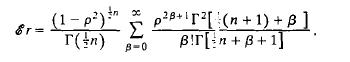
4.28. (Sec. 4.2) Prove[Him: Use Problem 4.26 and the duplication formula for the gamma function.] (1-p)*" (n) Wi 8-0 p28+ (n+1)+ B ] BIT+B+1] n
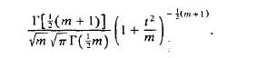
4.27. (Sec. 4.2) The I-distribution. Prove that if X and Yare independently distributed, X having the distnbution N(O,1) and Y having the X2-distribution with m degrees of freedom, then W = XI JY 1m has the density[Hint: In the joint density of X and Y, let x = tw1m- J: and integrate out w.]
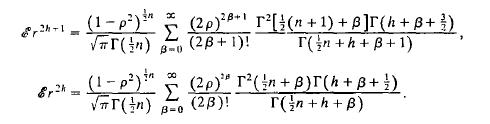
4.26. (Sec. 4.2) Prove for integer h 2h-1 (1-p) (2p)+ [ (n + 1) + ](h++ ) (n) (2+1)! 3-0 T(n + h + B + 1) (1-p) = 00 (n) (2B)! B-0 (2p) (n+B) ( h + B + } ) (n+h+B)
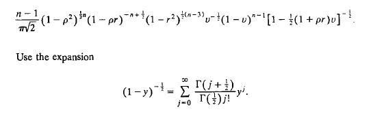
4.25. (Sec. 4.2) Prove that (40) is the density d r. [Hint: In (31) let all = ue-L' and a22 = ueu; show that the density of v (0 ~ v Show that the integral is (40).] n 2 (1-p) (1 - p)+(1 r ) v (1 v) [1 }(1 + pr}v]}. Use the expansion 00 (1-y)-(+) = j-0 T()!
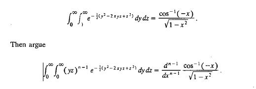
4.24. (Sec. 4.2) Prove that (39) is the density of r. [Hint: From Problem 2.12 showFinally show that the integral of(31) with respect to a II (= y 2 ) and a 22 (= z') is (39).] e-(y-2xyz+z) dydz = cos(-x) 1-x Then argue (yz)ey-2xyz+z2) dy dz d- cos(x) dx"-1
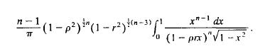
4.23. (Sec. 4.2.2) Prove that the density of the sample correlation r [given by(38)] is[Hint: Expand (1 - prx)-n in a power series, integrate, and use the duplication formula for the gamma ft:,nction.] n -(1-)(1)(-3)- x"-1 dx (1-pmx)"1-x
4.22. (Sec. 4.2.2) Prove Up) and f2( p) are monotonically increasing functions of p.
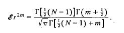
4.21. (Sec. 4.2.1) Prove that if p = 0 8,2m = T[(N-1)](m+) (N-1)+m]
4.20. (Sec. 4.2) Prove that if l: is diagonal, then the sets rij and aii are independently distributed. [Hint: Use the facts that rij is invariant under scale transformations and that the density of the observations depends only on the aii.]
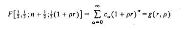
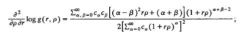
4.19. (Sec. 4.2) Prove r has a monotone likelihood ratio for r > 0, P > 0 by proving her) = kN(r, PI)/kN(r, P2) is monotonically increasing for PI > P2' Here her) is a constant times O:~:;:~Oca prra)/(r::~Oca pfra). In the numerator of h'(r), show that the coefficient of r {3 is positive. '
4.18. (Sec. 4.2) Show that of all tests of P = Po against p> Po based on r, a procedure for which r> c implies rejection is uniformly most powerful.
4.17. (Sec.4.2) Show that of all tests of Po against a specific PI (> Po) based on r, the procedures for which r> c implies rejection are the best. [Hint: This follows from Problem 4.16.]
4.16. (Sec. 4.2) Let kN(r, p) be the density of the sample corrclation coefficient r for a given value of P and N. Prove that r has a monotone likelihood ratio; that is, show that if PI > P2' then kN(r, PI)/kN(r, P2) is monotonically increasing in r. [Hint: Using (40), prove that ifhas a
4.15. (Sec. 4.2.2). Prove that when N = 2 and P = 0, Pr{r = l} = Pr{r = -l} = !.
4.14. (Sec. 4.2.3) Use Fisher's z to obtain a confidence interval for p with confidence 0.95 based on a sample correlation of 0.65 and a sample size of 25.
4.13. (Sec.4.2.3) Use Fisher's z to estimate P based on sample correlations of -0.7(N = 30) and of - 0.6 (N = 40).
4.12. (Sec. 4.2.3) Use Fisher's z to test the hypothesis PI = P2 against the alternatives PI *" P2 at the 0.01 level with rl = 0.5, NI = 40, r2 = 0.6, Nz = 40.
4.11. (Sec. 4.2.3) Use Fisher's Z to test the hypothesis P = 0.7 against alternatives {' *" O.i at the 0.05 level with' r = 0.5 and N = 50.
4.10. (Sec. 4.2:2) Suppose N = 10, , = 0.795. Find a one-sided confidence interval for p [of the form ('0,1)] with confidence coefficient 0.95.
4.9. (Sec. 4.2.2) Using the data of Problem 3.1, find a (two-sided) confidence interval for P12 with confidence coefficient 0.99.
4.8. (Sec. 4.2.2) Tablulate the power function at p = -1(0.2)1 for the tests in Problem 4.6. Sketch the graph of each power function.
4.7. (Sec. 4.2.2) Tablulate the power function at p = -1(0.2)1 for the tests in Problf!m 4.5. Sketch the graph of each power function.
4.6. (Sec. 4.2.2) Find significance points for testing p = 0.6 at the 0.01 level with N = 20 observations against alternatives (a) p *- 0.6, (b) p> 0.6, and (c) p < 0.6.
4.5. (Sec. 4.2.0 Find the significance points for testing p = 0 at the 0.01 level with N = 15 observations against alternatives (a) p *- 0, (b) p> 0, and (c) p < O.
4.4. (Sec. 4.2.2) Suppose a sample correlation of 0.65 is observed in a sample of 20.Test the hypothesis that the population correlation is 0.4 against the alternatives that the population correlation is greater than 0.4 at significance level 0.05.
4.3. (Sec. 4.2.1) Suppose a sample correlation of 0.65 is observed in a sample of 10.Test the hypothesis of independence against the alternatives of positive correlation at significance level 0.05.
4.2. (Sec. 4.2.1) Using the data of Problem 3.1, test the hypothesis that Xl and X2 are independent against all alternatives of dependence at significance level 0.01.
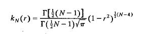
4.1. (Sec. 4.2.1) Sketchfor (a) N = 3, (b) N = 4, (c) N = 5, and (d) N = 10. KN(r)= [(N-1)] (N-1) (1-2) (N-4)
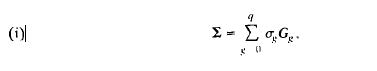
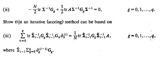
3.24. (Sec. 3.2) Covariance matrices with linear structure [Anderson (1969)]. Letwhere GO"'" Gq are given symmetric matrices such that there exists at least one (q + 1)-tuplet uo, u I ,. .. , uq such that (j) is positive definite. Show that the likelihood equations based on N observations are (i) 9
3.23. Let Z(k) = (Zij(k», where i = 1, ... , p. j = 1. ... , q and k = 1. 2..... be a sequence of random matrices. Let one norm of a matrix A be N1(A) =max i . j mod(a), and another he N2(A) = L',j a~ = tr AA'. Some alternative ways of defining stochastic convergence of Z(k) to B (p x q) are(a)
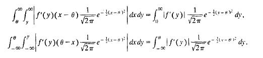
3.22. (Sec. 3.5) Show that 0) 1 dx dy == f'(y)\ x-(ro (x). LS(y) (8x) 1 2 - dy, 1- dy.
3.21. (Sec. 3.5) Demonstrate Lemma 3.5.1 using integration by parts.
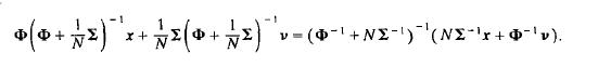
3.20. (Sec. 3.4) Show that P = = ( + N')' (N'r+'v). 1 (34+0)34+ (34+0)0 1-
3.19. (Sec. 3.4) Prove (l/N)L~_l(Xa - .... )(Xa - .... )' is an unbiased estimator of I when .... is known.
3.18. (Sec. 3.4) Prove l_~(~+l:)-l =l:(41+.l:)-1,~_~(~+l:)-l~=(~-l +l:-l)-l.113
3.17. (Sec. 3.2) Prove that Pr{IAI = O} = 0 for A defined by (4) when N > p. [Hint:Argue that if Z; = (ZI"'" Zp), then Iz~1 "" 0 implies A = Z;Z;' +r.;::p\ 1 ZaZ~ is positive definite. Prove Pr{l ztl = Zjjl zt-II + r.t::11 Zij cof(Zij)= O} = 0 by induction, j = 2, ... , p.]
3.16. {Sec. 3.3) Prove that i and S have efficiency [(N -l)/N]p{p+I)/2 for estimating jl. and l:.
3.15. G'ec.. 3.3) Efficiency of the mean. Prove that i is efficient for estimating jl..
3.14. (Sec. 3.3) Prove that the power of the test in (J 9) is a function only of p and[NI N2/(NI + N2)](jl.(11 - jl.(21),l: -1(jl.(11 - jl.(21), given VI.
3.13. (Sec. 3.3) Let Xa be distributed according to N( 'Yca, l:), a = 1, ... , N, where r.c~ > O. Show that the distribution of g = (l/r.c~)r.caXa is N[ 'Y,(l/r.c~)l:].Show that E = r.a(Xa - gcaXXa - gca)' is independently distributed as r.~.::l ZaZ~, where ZI'"'' ZN are independent, each with
3.12. (Sec. 3.2) Prove Lemma 3.2.2 by using Lemma 3.2.3 and showing N log I CI -tr CD has a maximum at C = ND -I by setting the derivatives of this function with respect to the elements of C = l: -I equal to O. Show that the function of C tends to -00 as C tends to a singular matrix or as one or
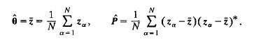
3.11. (Sec. 3.2) Estimation of parameters of a complex normal distribution. Let ZI"'" ZN be N obseIVations from the complex normal distributions with mean 6 and covariance matrix P. (See Problem 2.64.)(a) Show that the maximum likelihood estimators of 0 and Pare(b) Show that Z has the complex
3.10. (Sec. 3.2) Estimation of l: when jl. is known. Show that if XI"'" XN constitute a sample from N(jl., l:) and jl. is known, then (l/N)r.~_I(Xa - jl.XXa - jl.)' is the maximum likelihood estimator of l:.
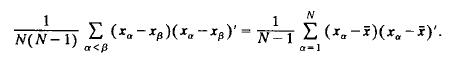
3.9. (Sec. 7.2) Show that(Note: When p = 1, the left-hand side is the average squared differences of the observations.) N N(N-1)(x-x) (x-x)'=(x*)(**)'.
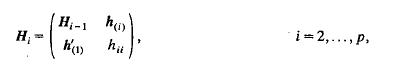
3.8. (Sec. 3.2) Prove Lemma 3.2.2 by induction. [Hint: Let HI = h ll ,and use Problem 2.36.] H-1 h i-2,..., p. H h' (1) hii
3.7. (Sec. 3.2) In variance of the sample correlation coefficient. Prove that r 12 is an invariant characteristic of the sufficient statistics i and S of a bivariate sample under location and scale transformations (Xfa = bix;a + Ci' bi> 0, i = 1,2, a =1, ... , N) and that every function of i and S
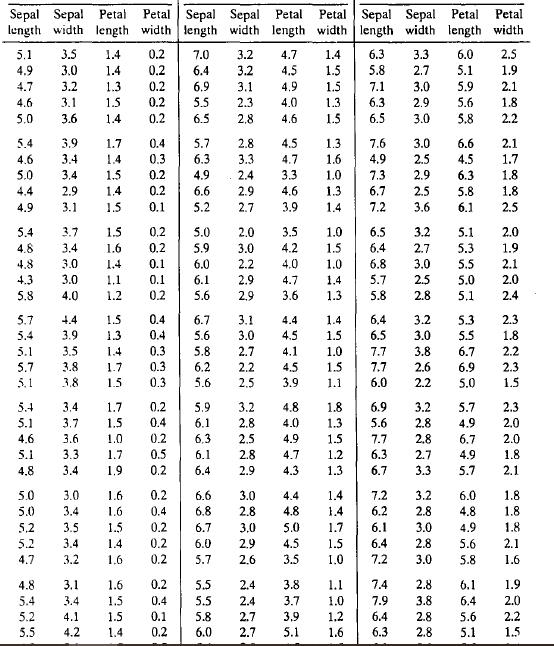
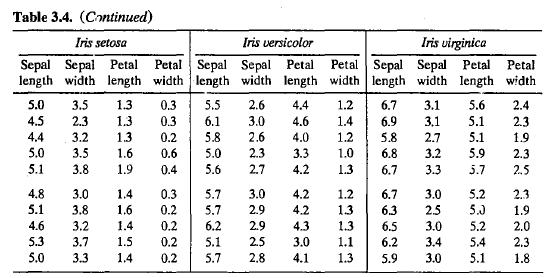
3.6. Find fL, 1:, and ( P;j) for Iris setosa from Table 3.4, taken from Edgar Anderson's famous iris data [Fisher (1936)].
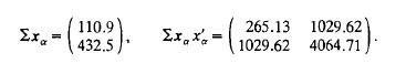
3.5. (Sec. 3.2) Let Xl be the body weight (in kilograms) of a cat and X2 the heart weight (in grams). [Data from Fisher (1947b).](a) In a sample of 47 female cats the relevant data areFind jl, t, S, and p.(b) In a sample of 97 male cats the relevant data areFind fL, l;, S, and p. 110.9 (432.5) =
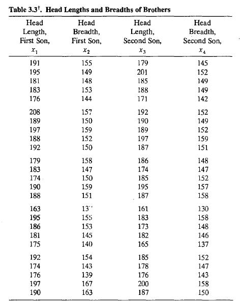
3.4. (Sec. 3.2) Use the facts that I C* I = n A;, tr C* = ~Ai' and C* = I if Al = ...= Ap = 1, where AI' ... ' Ap are the characteristic roots of C*, to prove Lemma 3.2.2. [Hint: Use f as given in (12).) Table 3.3'. Head Lengths and Breadths of Brothers Head Length, Head Breadth, Head Length, First
3.3. (Sec. 3.2) Compute ji, i, S, and P for the following pairs of observations:(34,55), (12, 29), (33, 75), (44, 89), (89, 62), (59, 69), (50, 41), (88, 67). Plot the observations.
3.2. (Sec. 3.2) Verify the numerical results of (21).
3.1. (Sec. 3.2) Find ji, i, and (Pi}) for the data given in Table 3.3, taken from Frets (1921).
2.68. (Sec. 2.7) For the multivariate I-distribution with density (41) show that GX= V- and C(X) = [m/(m - 2)]
2.67. (Sec. 2.2) Show that f''-.e-x'/2dx/& is approximately (l_e- 2a'/,,)1/2.[Hint: The probability that (X, Y) falls in a square is approximately the probability that (X, Y) falls in an approximating circle [P6lya (1949)].]
2.66. Show that the characteristic function of Z defined in Problem 2.64 iswhere l?ll(x + iy) = x. ER(Z)=eu-u* Pu
2.65 • Complex no/mal (continued). If Z has the complex normal distribution of,,"' Problem 2.64, show that W = AZ, where A is a nonsingular complex matrix, has the complex normal distribution with mean AS and covariance matrix C(W) =, APA*.
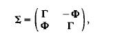
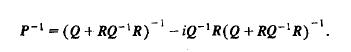
2.64. Complex normal distribution. Let (X', Y')' have a normal distribution with mean vector (,ix, ,iy)' and covariance matrixwhere f is positive definite and III = - III' (skew symmetric). Then. Z = X + iY is said to have a complex normal distribution with mean 6 = I~x +il J.y and covariance
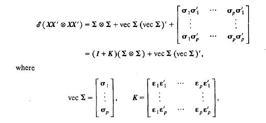
2.63. (Sec. 2.6) Suppose X is distributed according to N(o, I). Let 1= (0"1"'" O"p)'Proveand E; is a column vector with 1 in the ith position and O's elsewhere. where (XX' XX')=+ vec (vec )' + = (1 + )( ) + vec (vec )', vec - = K
2.62. (Sec. 2.6) Let the density of (X, Y) be 2n(xIO, l)n(yIO, 1), O!>y!>x < 00, O!> -x!>y < 00, O!> -y!> -xx!> -y
2.61. (Sec. 2.6) Verify (25) and (26) by using the transformation X - IJ. = CY, where 1= CC', and integrating the density of Y.
2.60. (Sec. 2.6) Let Y be distributed according to N(O, I). Differentiating the characteristic function, verify (25) and (26).
2.59. (Sec. 2.6) Prove Lemma 2.6.2 in detail. '"
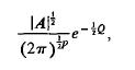
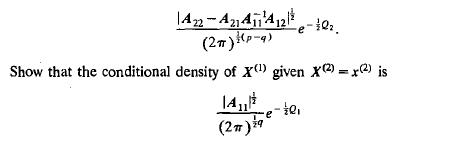
2.58. (Sec. 2.5) Suppose X(I) and X(2) of q and p - q components, respectively, have the densitywhere Q = (xO) - fL(I») , A II ( x(l) - fL(I») + (x(l) - fL(I») , A 12 ( x(2) - fL(2»)+ ( X(2) - fL(2») , A 21( x(l) - fLO») + (X(2) - fL(2») , An( X(2) - fL(2»).Show that Q can be written as QI
2.57. (Sec. 2.5) Inuariance of the partial correlation coefficient. Prove that P12.3, ... , P. is invariant under the transformations xi = ajxj + b;X(3) + cj ' a j > 0, i = 1,2, x(3)*= ex(3) +d, where x(3) = (x3, ••. , xp )', and that any function of fL and I that is invariant under these
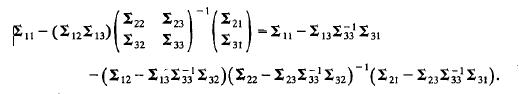
2.56. (Sec. 2.5) Prove by matrix algebra that (22 23 F11-(2 12213) 232 233) 11-(21213) 21 1) - - 31 -(12-1323332) (22-233332)(21-22323331).
2.55. (Sec. 2.5) Show c8'( x(I)lxt2), x(3») = fL(l) + I 13I;:l (X(3) - fL(3»)+ (I12 - II3I 331 I 32 )( I22 - I23 I 331 I 32r l. [ X(2) - fL(2) - I23 I ;} (X(3) - fL(3»)] .
2.54. (Sec. 2.5) Use Problem 2.53 to show that x'I -IX = (X(I) - I12Ii2IX(2»)'I'/2( x(1) - I12Ii2IX(2») + x(2)'Iib(2).
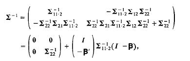
2.53. (Sec. 2.5) Showwhere 13 = I12Iit [Hint: Use Theorem A.3.3 of the Appendix and the fact that I -1 is symmetric.] 0 -1 11-2 21-11-2 I - 11-2124 22 5- 2111 212 -B' (1 - 1),
2.52. (Sec. 2.5) Verify that I12Ii21 = -"'Ill "'12' where'" = I-I is partitioned similarly to I.
2.51. . (Sec. 2.5) Show that for any vector functicn h(x(2»)is positive semidefinite. Note this generalizes Theorem 2.5.3 and Problem 2.49. [x-h(x)][x-(x)]' - [x - &X\X][x - $x[x]'
2.50. (Sec. 2.5) Show that for any function h(X(2» and any joint distribution of Xi and X(2) for which the relevant expectations exist, the correlation between Xi and h(X(2») is not greater than the correlation between Xi and g(X(2»), where g(X(2») = J' Xilx(2).
2.49. (Sec. 2.5) Show that for any function h(X(2») and any joint distribution of Xi and Xl2l for which the relevant expectations exist, J'[Xi - h(X{2))f = J'[Xi -g(X(2»)]2 + J'[g(X(2») - h(X(2»)]2, where g(X(2») = J'Xj IX(2) is the conditional expectation of Xi given X(2) = x(2). Hence
2.48. (Sec. 2.5) Show that for any joint distribution for which the expectations exist and any function h( X(2») tha t[Hiw: In the above take the expectation first with respect to Xi conditional 011 X(2).] (XXX)) h(x()) = 0.
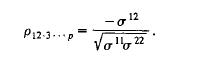
2.47. (Sec. 2.5) Prove[Hint: Apply Theorem A.3.2 of the Appendix to the cofactors used to calculate u~ . P12-3-p 12 1122
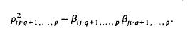
2.46. (Sec. 2.5) Show 2 Pg+1 p = Bijg+1p Bj.q+1,....p ......
Showing 3000 - 3100
of 5397
First
24
25
26
27
28
29
30
31
32
33
34
35
36
37
38
Last
Step by Step Answers