New Semester Started
Get
50% OFF
Study Help!
--h --m --s
Claim Now
Question Answers
Textbooks
Find textbooks, questions and answers
Oops, something went wrong!
Change your search query and then try again
S
Books
FREE
Study Help
Expert Questions
Accounting
General Management
Mathematics
Finance
Organizational Behaviour
Law
Physics
Operating System
Management Leadership
Sociology
Programming
Marketing
Database
Computer Network
Economics
Textbooks Solutions
Accounting
Managerial Accounting
Management Leadership
Cost Accounting
Statistics
Business Law
Corporate Finance
Finance
Economics
Auditing
Tutors
Online Tutors
Find a Tutor
Hire a Tutor
Become a Tutor
AI Tutor
AI Study Planner
NEW
Sell Books
Search
Search
Sign In
Register
study help
business
probability statistics
Modern Statistics For The Social And Behavioral Sciences 2nd Edition Rand Wilcox - Solutions
In the previous exercise, you could have used averages rather than difference scores when comparing the murderers to the controls. That is, the hypothesis given by Equation (11.10) could have been tested. Using the R function sppba with the argument avg set equal to TRUE, verify that the p-value is
Using the data in Exercise 1, test Equation (11.9) using a one-step M-estimator via the R function sppba. Verify that the p-value is 0.06.
The last example in Section 11.6.6 described a study comparing EEG measures for murderers to a control group. The entire data set, containing measures taken at four sites in the brain, can be downloaded from the author’s web page as described in Chapter 1 and is stored in the file eegall.dat. The
Repeat the illustration in Section 10.5.1, but now compare the groups using the modified one-step M-estimator via the R function pbad2way. Verify that for Factor B, now the p-value is 0.059. How does this compare to the results using a 20% trimmed mean? Note: the data can be read into R as
For the data in Exercise 10, verify that if t2way is used to compare 20% trimmed means, the p-values for Factors A and B are 0.145 and 0.93. Why does the p-value for Factor A drop from 0.372 when comparing means to 0.145 with 20% trimmed means instead?
For the data in the previous exercise, verify that if t2way is used to compare 20% trimmed means, the p-value when testing the hypothesis of no interaction is reported to be 0.408.
The file CRCch10 Ex10.txt, stored on the author’s web page, contains data, the first few lines of which look like this:The first two columns indicate the levels of two factors and the dependent variable is in colume 3.Use the function t2way to test the hypotheses of no main effects or
Verify that when comparing the groups in Table 10.1 based on medians and with the R function pbad2way in Section 10.4.1, the p-values for Factors A and B are 0.28 and 0.059, respectively, and that for the test of no interaction, the significance level is 0.13.
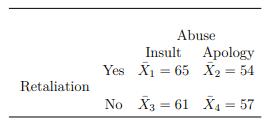
This exercise is based on a study by Atkinson and Polivy where the general goal was to study people’s reactions to unprovoked verbal abuse. In the study, 40 participants were asked to sit alone in a cubicle and answer a brief questionnaire.After waiting far longer than it took to fill out the
Referring to Exercise 5, imagine the hypothesis of no interactions is rejected. Is it reasonable to conclude that the interaction is disordinal?
In the previous exercise, suppose the hypothesis of no interactions is rejected and in fact there is a disordinal interaction. What does this suggest about using method 1 rather than method 2?
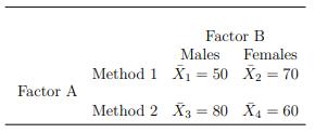
Imagine a study where two methods are compared for treating depression. A measure of effectiveness has been developed, the higher the measure the more effective the treatment. Further assume there is reason to believe that males might respond differently to the methods compared to females. If the
Make up an example where the population means in a 3-by-3 design have no interaction effect but main effects for both factors exist.
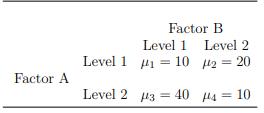
Consider a 2-by-2 design with population meansDetermine whether there is an interaction. If there is an interaction, determine whether there is an ordinal interaction for rows. Factor A Factor B Level 1 Level 2 Level 1 10 2=20 Level 2 3 40 4 = 10 =
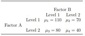
Consider a 2-by-2 design with population meansState whether there is a main effect for Factor A, for Factor B, and whether there is an interaction. Factor A Factor B Level 1 Level 2 Level 1 110 2= 70 Level 2 3 80 4= = 144 40
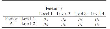
For a 2-by-4 design with population meansstate the hypotheses of no main effects and no interactions. Factor B Level 1 Level 2 level 3 Level 4 Factor Level 1 12 3 144 A Level 2 145 146 147 148
Repeat the last exercise, only now use projection distances by setting the argument op=3. Verify that the p-value is 0.004. Why does op=3 avoid the error noted in the last exercise?
For the data in Table 9.6, use pbadepth to compare the groups using default values for the arguments. You will get the message:Error in solve.default(cov, ...) :system is computationally singular:reciprocal condition number = 2.15333e-18 The difficulty is that the depth of the null vector is being
For the data in Table 9.6, use t1way to compare 20% trimmed means and verify that the p-value is less than 0.01.
For the data in Table 9.6, verify that the p-value, based on Welch’s test, is 0.98.Use the R Function t1way. (The data are stored on the author’s web page in the file ch9 table9 6 dat.txt.)
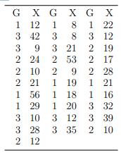
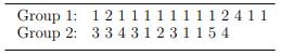
Consider the following data.Store this data in an R variable having matrix mode with two columns corresponding to the two variables shown. (The data are stored on the author’s web page in the file ch9 ex14 dat.txt.) There are three groups with the column headed by G indicating to which group the
Repeat the last exercise, but now use projection distances to measure the depth of the null vector. That is, set the argument op=3.
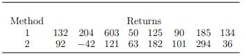
For the data in Table 9.1, use method LSPB to compare the groups using the modified one-step M-estimator, MOM. Compare the p-value to what you get when using a 20% trimmed mean instead. What does this illustrate?
For the data in Table 9.1, the ANOVA F test and Welch’s test were not significant with α = 0.05. Imagine that you want power to be 0.9 if the mean of one of the groups differs from the others by 0.2. (In the notation of Section 9.3, a = 0.2.)Verify that according to the R function bdanova1, the
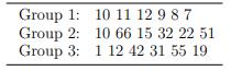
For the following data, use R to verify that you do not reject with the ANOVA F testing with α = 0.05, but you do reject with Welch’s test.What might explain the discrepancy between the two methods? Group 1: 10 11 12 987 Group 2: 10 66 15 32 22 51 Group 3: 112 42 31 55 19
Consider J = 5 groups with population means 3, 4, 5, 6, and 7, and a common variance σ2 p = 2.If n = 10 observations are sampled from each group, determine the value estimated by MSBG and comment on how this differs from the value estimated by MSWG.
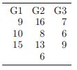
Using R, verify that for the following data, MSBG = 14.4 and MSWG = 12.59. G1 10 G2 G3 9 16 7 8 15 13 6 691
For the data in Table 9.1, assume normality and that the groups have equal variances. As already illustrated, the hypothesis of equal means is not rejected.If the hypothesis of equal means is true, an estimate of the assumed common variance is MSBG = 0.12, as already explained. Describe a reason
For the datastore the data in an R variable having list mode and and use the R function anova1 to verify that when using the ANOVA F test, the estimate of the assumed common variance is MSWG = 9.5. Next, compute MSWG using the R function lapply and the R function list2matrix, which converts data in
For the data in Exercise 1, verify that when comparing 20% trimmed means with the R function t1way, the p-value is 0.02.
For the data in Exercise 1, verify that Welch’s test statistic is Fw = 7.7 with degrees of freedom ν1 = 2 and ν2 = 13.4. Using the R function t1way, verify that you would reject the hypothesis of equal means with α = 0.01.
For the data in the previous exercise, test the hypothesis of equal means using the ANOVA F. Use α = 0.05. Verify that MSBG = 25.04, MSWG=4.1369 , F = 6.05, and that you reject at the 0.05 level. Check your results using R. The data are stored in file CH9ex1.txt on the author’s web page, which
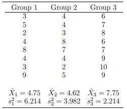
For the following data,assume that the three groups have a common population variance, σ2 p . Estimate σ2 p . Group 1 3 35249 8 Group 2 Group 3 4 4 3 8 10 69867999 7425 X = 4.75 X2 = 4.62 X2 4.62 X3 = 7.75 s=6.214 $23.982 $ = 2.214
Repeat the previous exercise, only now compare the marginal 20% trimmed means using the R function yuend with the argument tr=0.2. Verify that the p-value is 0.2209.
The file scent dat.txt, stored on the author’s web page, contains data downloaded from a site maintained by Carnegie Mellon University. Read the file into an R variable called scent. The last six columns contain the time participants required to complete a pencil and paper maze when they were
Continuing the last exercise, plot the difference scores using the R function akerd and note that the distribution is skewed to the right, suggesting that the confidence interval for the mean might be inaccurate. Using the R function trimcibt, verify that the 0.95 confidence interval for the 20% of
Section 8.2.1 analyzed the Indometh data stored in R using the R function trimci. Compare times 2 and 3 using means based on difference scores and verify that the p.value is 0.014.
For two dependent groups you getApply the Wilcoxon signed rank test with α = 0.05. Verify that W = 0.7565 and that you fail to reject. Group 1: 86 71 Group 2: 88 77 77 68 91 72 77 91 70 71 88 87 76 64 96 72 65 90 65 80 81 72
For two dependent groups you getCompare the two groups with the sign test and the Wilcoxon signed rank test with α = 0.05. Verify that, according to the sign test, ˆp = 0.29 and that the 0.95 confidence interval for p is (0.04, 0.71), and that the Wilcoxon signed rank test has an approximate
Repeat the last exercise, only now use a 20% trimmed mean. Verify that the p-value is 0.049.
Repeat Exercise 1, but now use a bootstrap-t method via the R function trimcibt. Verify that the p-value is 0.091.
Is it possible that the marginal trimmed means are equal but the trimmed mean based on the difference scores is not equal to zero? What does this indicate in terms of power?
Generally, why is it possible to get a different p-value comparing the marginal trimmed means versus making inferences about the trimmed mean of the difference scores?
If in Exercise 1 you compare the marginal 20% trimmed means with the R function yuend, verify that now the p-value is 0.121.
Repeat the previous exercise, but use 20% trimmed means instead using the difference scores in conjunction with the R function trimci. Verify that the pvalue is 0.049.
For the data in Table 8.1, perform the paired T test for means using the weights for the east and south sides of the trees. Verify that the p-value is 0.44.
R contains data, stored in the R variable sleep, which show the effect of two soporific drugs, namely the increase in hours of sleep compared to control. Create a boxplot for both groups using the command boxplot(sleep[[1]] ∼ sleep[[2]]) and speculate about whether comparing 20% trimmed means
For the data in the previous exercise, verify that the p-value based on Cliff’s method is 0.01 and for the Brunner–Munzel method the p-value is less than 0.001.
Two independent groups are given different cold medicines and the goal is to compare reaction times. Suppose that the decreases in reaction times when taking drug A versus drug B are as follows.A: 1.96, 2.24, 1.71, 2.41, 1.62, 1.93 B: 2.11, 2.43, 2.07, 2.71, 2.50, 2.84, 2.88 Verify that the
Imagine that two groups of cancer patients are compared, the first group having a rapidly progressing form of the disease and the other having a slowly progressing form instead. At issue is whether psychological factors are related to the progression of cancer. The outcome measure is one where
Two methods for reducing shoulder pain after laparoscopic surgery were compared by Jorgensen et al. (1995). The data wereVerify that both the Wilcoxon–Mann–Whitney test and Cliff’s method reject at the 0.05 level. Although the Kolmogorov–Smirnov test rejects with α = 0.05, why might you
The last example in Section 7.5.5 dealt with comparing males to females regarding the desired number of sexual partners over the next 30 years. Using Student’s T, we fail to reject which is not surprising because there is an extreme outlier among the responses given by males. If we simply discard
For the data in Table 7.4, verify that the 0.95 confidence interval for the difference between the biweight midvariances is (−154718, 50452).
Describe a general situation where comparing medians will have more power than comparing means or 20% trimmed means.
For the data in Table 7.5, use the R function comvar2 to verify that the 0.95 confidence interval for the difference between the variances is (−1165766.8, 759099.7).
For the self-awareness data in Table 7.5, verify that the R function yuenbt, with the argument tr set to 0, returns (−571.4, 302.5) as a .95 confidence interval for the difference between the means.
Create a boxplot of the data in Table 7.6 and comment on why the probability coverage, based on Student’s T or Welch’s method, might differ from the nominalα level.
The 20% Winsorized standard deviation (sw) for the first group in Table 7.6 is 1.365 and for the second group it is 4.118. Verify that the 0.95 confidence interval for the difference between the 20% trimmed means, using Yuen’s method, is (5.3, 22.85).
In the previous exercise you do not reject the hypothesis of equal variances. Why is this not convincing evidence that the assumption of equal variances, when using Student’s T, is justified?
For the data in Table 7.6, the are 0.95 confidence interval for the difference between the means based on Welch’s method is (1.96, 20.83). Check this result with the R function yuen.
Student’s T rejects the hypothesis of equal means based on the data in Table 7.6.Interpret what this means.
Verify that the 0.95 confidence interval for the difference between the means, based on the data in Table 7.6 and Student’s T, is (2.2, 20.5). What are the practical concerns with this confidence interval?
The sample means for the data in Table 7.6 are 22.4 and 11.If we test the hypothesis of equal means using Student’s T, verify that T = 2.5 and that you would reject with α = 0.05.
For the data in Table 7.6, if we assume that the groups have a common variance, verify that the estimate of this common variance is s 2p = 236.
In the previous exercise, you rejected the hypothesis of equal means. What does this imply about the accuracy of the confidence interval for the difference between the population means based on Student’s T?
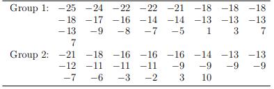
Published studies indicate that generalized brain dysfunction may predispose someone to violent behavior. Of interest is determining which brain areas might be dysfunctional in violent offenders. In a portion of such a study conducted by Raine, Buchsbaum, and LaCasse (1997), glucose metabolism
Use Cohen’s d to measure effect size using the data in the previous two exercises.
Repeat the previous exercise, only use Yuen’s test with 20% trimmed means.
Responses to stress are governed by the hypothalamus. Imagine you have two groups of participants. The first shows signs of heart disease and the other does not. You want to determine whether the groups differ in terms of the weight of the hypothalamus. For the first group of participants with no
You compare lawyers versus professors in terms of job satisfaction and fail to reject the hypothesis of equal means or equal trimmed means. Does this mean it is safe to conclude that the typical lawyer has about the same amount of job satisfaction as the typical professor?
Repeat the last exercise, only compare 20% trimmed means instead.
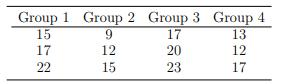
Two methods for training accountants are to be compared. Students are randomly assigned to one of the two methods. At the end of the course, each student is asked to prepare a tax return for the same individual. The returns reported by the students areUsing Welch’s test, would you conclude that
Repeat the last exercise, only use Student’s T instead.
For X¯1 = 10, X¯2 = 5, s 21 = 21, s 22 = 29, n1 = n2 = 16, compute a 0.95 confidence interval for the difference between the means using Welch’s method and state whether you would reject the hypothesis of equal means.
Referring to the last exercise, compute a 0.99 confidence interval for the difference between the trimmed means.
If for two independent groups, you get X¯t1 = 42, X¯t2 = 36, s 2w1 = 25, s 2w2 = 36, n1 = 24, and n2 = 16, test the hypothesis of equal trimmed means with α = 0.05.
Comparing the results of the last two exercises, what do they suggest about using Student’s T versus Welch’s method when the sample variances are approximately equal?
Repeat the last exercise using Welch’s method.
For two independent groups of subjects, you get X¯1 = 86, X¯2 = 80, s 21 = s 22 = 25, with sample sizes n1 = n2 = 20.Assume the population variances of the two groups are equal and verify that Student’s T rejects with α = 0.01.
Comparing the test statistics for the last two exercises, what do they suggest regarding the power of Welch’s test versus Student’s T test for the data being examined?
Repeat the last exercise, only use Welch’s test for comparing means.
Still assuming equal variances, test the hypothesis of equal means using the data in the last exercise assuming random sampling from normal distributions. Useα = 0.05.
For two independent groups of subjects, you get X¯1 = 45, X¯2 = 36, s 21 = 4, s 22 = 16 with sample sizes n1 = 20 and n2 = 30.Assume the population variances of the two groups are equal and verify that the estimate of this common variance is 11.25.
Suppose that the sample means and variances are X¯1 = 15, X¯2 = 12, s 21 = 8, s 22 = 24 with sample sizes n1 = 20 and n2 = 10.Verify that s 2p = 13.14, T = 2.14 and that Student’s T test rejects the hypothesis of equal means with α = 0.05.
R has a built-in dataset called leuk. The third column indicates survival times of patients diagnosed with acute myelogenous leukemia. The first column indicates the patient’s white blood cell count at the time of diagnosis. Using least squares regression, assuming homoscedasticity, test the
To illustrate a point, assume that for the data in Table 6.9, the goal is to predict X given Y, rather than predict Y given X. Use the R functions ols and rqfit to test the hypothesis H0 : β1 = 0 with α = 0.05. Verify that ols fails to reject, its p-value is approximately 0.97, but rqfit rejects.
Verify that for the data in Table 6.6, when testing the hypothesis of homoscedasticity using the R function khomreg, you fail to reject with α = 0.05. Explain why this result is not a satisfactory reason for assuming homoscedasticity.
The data in Table 6.9 are from a study, conducted by L. Doi where the goal is to understand how well certain measures predict reading ability in children. Verify that the 0.95 confidence interval for the slope is (−0.16, .12) based on Equation(6.8).
Suppose you observe X: 12.2, 41, 5.4, 13, 22.6, 35.9, 7.2, 5.2, 55, 2.4, 6.8, 29.6, 58.7 Y : 1.8, 7.8, 0.9, 2.6, 4.1, 6.4, 1.3, 0.9, 9.1, 0.7, 1.5, 4.7, 8.2 Verify that the 0.95 confidence interval for the slope is (0.14, 0.17). Would you reject H0 :β1 = 0? Based on this confidence interval only,
You measure stress (X) and performance (Y ) on some task and get X : 18 20 35 16 12 Y : 36 29 48 64 18Verify that you do not reject H0 : β1 = 0 using α = 0.05. Is this result consistent with what you get when testing H0 : ρ = 0? Why would it be incorrect to conclude that X and Y are independent?
Imagine two scatterplots, where in each scatterplot the points are clustered around a line having slope 0.3. If for the first scatterplot r = 0.8, does this mean that points are more tightly clustered around the line versus the other scatterplot where r = 0.6?
For the data in Exercise 17, the sizes of the corresponding lots are:18,200 12,900 10,060 14,500 76,670 22,800 10,880 10,880 23,090 10,875 3498 42,689 17,790 38,330 18,460 17,000 15,710 14,180 19,840 9150 40,511 9060 15,038 5807 16,000 3173 24,000 16,600.Verify that the least squares regression
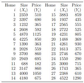
The selling price and size of a home for a suburb of Los Angeles in the year 1997 are shown in Table 6.8. At the time, even a small empty lot would cost at least$200,000. Verify that based on the least squares regression line for these data, if we estimate the cost of an empty lot by setting the
For the data in Exercise 15, verify that a least squares regression line using only X values (age) less than 7 yields b1 = 0.247 and b0 = 3.51. Verify that when using only the X values greater than 7 you get b1 = 0.009 and b0 = 4.8. What does this suggest about using a linear rule for all of the
Sockett et al. (1987) report data related to patterns of residual insulin secretion in children at the time they were diagnosed with diabetes. A portion of the study was concerned with whether age can be used to predict the logarithm of C-peptide concentrations at diagnosis. The observed values are
Vitamin A is required for good health. You conduct a study and find that as vitamin A intake increases, certain health problems decrease. However, for levels of vitamin A not included in your study, a sufficiently high dose can result in death. Comment on what this illustrates in the context of
Repeat Exercise 12, only for the points X: 1 2 3 4 5 6 Y : 4 5 6 7 8 2
Verify that for the following pairs of points, the least squares regression line has a slope of zero. Plot the points and comment on the assumption that the regression line is straight.X: 1 2 3 4 5 6 Y : 1 4 7 7 4 1
Maximal oxygen uptake (mou) is a measure of an individual’s physical fitness. You want to know how mou is related to how fast someone can run a mile. Suppose you randomly sample six athletes and getCompute the correlation. Can you be reasonably certain about whether it is positive or negative
In Exercise 6, what would be the least squares estimate of the cancer rate given a solar radiation of 600? Indicate why this estimate might be unreasonable.
Showing 3000 - 3100
of 8686
First
24
25
26
27
28
29
30
31
32
33
34
35
36
37
38
Last
Step by Step Answers