New Semester Started
Get
50% OFF
Study Help!
--h --m --s
Claim Now
Question Answers
Textbooks
Find textbooks, questions and answers
Oops, something went wrong!
Change your search query and then try again
S
Books
FREE
Study Help
Expert Questions
Accounting
General Management
Mathematics
Finance
Organizational Behaviour
Law
Physics
Operating System
Management Leadership
Sociology
Programming
Marketing
Database
Computer Network
Economics
Textbooks Solutions
Accounting
Managerial Accounting
Management Leadership
Cost Accounting
Statistics
Business Law
Corporate Finance
Finance
Economics
Auditing
Tutors
Online Tutors
Find a Tutor
Hire a Tutor
Become a Tutor
AI Tutor
AI Study Planner
NEW
Sell Books
Search
Search
Sign In
Register
study help
business
probability statistics
Modern Statistics For The Social And Behavioral Sciences 2nd Edition Rand Wilcox - Solutions
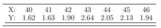
For the following data, compute the least squares regression line for predicting Y from X. X: 40 41 42 43 44 45 46 Y: 1.62 1.63 1.90 2.64 2.05 2.13 1.94 2.64 2.05
For the data in the last exercise, verify that the coefficient of determination is 0.36 and interpret what this tells you.
For the following data, compute the least squares regression line for predicting GPA given SAT. SAT: 500 530 590 660 GPA: 2.3 3.1 2.6 3.0 610 700 570 640 2.4 3.3 2.6 3.5
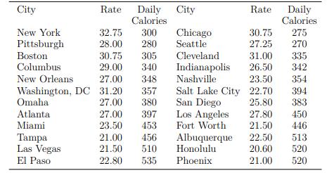
The following table reports breast cancer rates plus levels of solar radiation (in calories per day) for various cities in the United States. Fit a least squares regression to the data with the goal of predicting cancer rates and comment on what this line suggests. City Rate Daily City Calories
Verify that for the data in Table 6.3, the least squares regression line is Yˆ =−0.0405X + 4.581.
Suppose that based on n = 25 values, s 2x = 12, s 2y = 25, and r = 0.6. What is the slope of the least squares regression?
Verify that for the data in Exercise 1, if you use Yˆ = 2X − 9, the sum of the squared residuals is larger tha 47.Why would you expect a value greater than 47?
Compute the residuals using the results from Exercise 1.Verify that if you square and sum the residuals, you get 47, rounding to the nearest integer.
For the data in Exercise 37, compute a 0.95 confidence interval for the median using the R function sint described in Chapter 4.What does this suggest about using a median versus a one-step M-estimator?
For the data in Exercise 37, what practical problem might occur if the standard error of the median is estimated using a bootstrap method?
Repeat the last exercise, only now trim 40%. Verify that the 0.95 confidence interval is now (7.0, 14.5). Why is this confidence interval so much shorter than the confidence interval in the last exercise?
Use trimpb on the data used in the previous two exercises, but this time trim 30%.Verify that the 0.95 confidence interval for the trimmed mean is (7.125, 35.500).Why do you think this confidence interval is shorter versus the confidence interval in the last exercise?
For the data in the previous exercise, verify that the 0.95 confidence interval for the 20% trimmed mean returned by the R function trimpb is (7.25, 63). Why would you expect this confidence interval to be substantially longer than the confidence interval based on a one-step M-estimator?
For the following observations 2, 4, 6, 7, 8, 9, 7, 10, 12, 15, 8, 9, 13, 19, 5, 2, 100, 200, 300, 400 verify that the 0.95 confidence interval, based on a one-step M-estimator and returned by onesampb, is (7.36, 19.77).
Which of the two confidence intervals given in the last two exercises is likely to have probability coverage closer to 0.95?
For the data in Exercise 31, verify that the 0.95 confidence interval for the population 20% trimmed mean using trimpb is (9.75, 31.5).
For the data in Exercise 30, verify that the equal-tailed .95 confidence interval for the population 20% trimmed mean using trimcibt is (8.17, 15.75).
Referring to the previous two exercises, which confidence interval for the mean is more likely to have probability coverage at least 0.95?
For the data in the previous exercise, verify that the 0.95 confidence interval for the mean returned by the R function trimcibt is (12.40, 52.46). Note that the length of this interval is much higher than the length of the confidence interval for the mean using trimci.
Rats are subjected to a drug that might cause liver damage. Suppose that for a random sample of rats, measures of liver damage are found to be 5, 12, 23, 24, 6, 58, 9, 18, 11, 66, 15, 8.Verify that trimci returns a 0.95 confidence interval for the 20% trimmed mean, using R, equal to (7.16, 22.84).
For the following 10 bootstrap sample means, determine a p-value when testing the hypothesis H0: µ = 8.5.7.6, 8.1, 9.6, 10.2, 10.7, 12.3, 13.4, 13.9, 14.6, 15.2.What would be an appropriate 0.8 confidence interval for the population mean?
A standard measure of aggression in 7-year-old children has been found to have a 20% trimmed mean of 4.8 based on years of experience. A psychologist wants to know whether the trimmed mean for children with divorced parents differs from 4.8. Suppose X¯t = 5.1 with sw = 7 based on n = 25.Test the
For the data in Exercise 24, the trimmed mean is X¯t = 42.17 with a Winsorized standard deviation of sw = 1.73. Test the hypothesis that the population trimmed mean is 45 with α = 0.05.
Repeat the previous exercise, only test the hypothesis H0: µt < 42 with α = 0.05 and n = 16.
Given the following values for X¯t and sw: (a) X¯t = 44, sw = 9, (b) X¯t = 43, sw = 9, (c) X¯t = 43, sw = 3, and assuming 20% trimming, test the hypothesis H0: µt = 42 with α = 0.05 and n = 20.
A portion of a study by Wechsler (1958) reports that for 100 males taking the Wechsler Adult Intelligent Scale (WAIS), the sample mean and variance on picture completion are X¯ = 9.79 and s = 2.72. Test the hypothesis H0: µ ≥ 10.5 with α = 0.025.
A company claims that, on average, when exposed to its toothpaste, 45% of all bacteria related to gingivitis is killed. You run 10 tests and find that the percentages of bacteria killed among these tests are 38, 44, 62, 72, 43, 40, 43, 42, 39, 41.The mean and standard deviation of these values are
Repeat the previous exercise but only test H0: µ > 42.
Given the following values for X¯ and s: (a) X¯ = 44, s = 10, (b) X¯ = 43, s = 10,(c) X¯ = 43, s = 2, test the hypothesis H0: µ < 42 with α = 0.05 and n = 16.
For part b of the last exercise you fail to reject but you reject for the situation in partc. What does this illustrate about power?
Given the following values for X¯ and s: (a) X¯ = 44, s = 10, (b) X¯ = 43, s = 10,(c) X¯ = 43, s = 2, test the hypothesis H0: µ = 42 with α = 0.05 and n = 25.
For the previous exercise, rather than increase the sample size, what else might you do to increase power? What is a negative consequence of using this strategy?
The previous exercise indicates that power is relatively low with only n = 10 observations. Imagine that you want power to be at least 0.8. One way of getting more power is to increase the sample size, n. Verify that for sample sizes of 20, 30, and 40, power is 0.56, 0.71, and 0.81, respectively.
For the previous exercise, verify that power is 0.35 if µ = 46.
A manufacturer of medication for migraine headaches knows that its product can cause liver damage if taken too often. Imagine that by a standard measuring process, the average liver damage is µ = 48.A modification of the product is being contemplated, and based on n = 10 trials, it is found that
For n = 49, α = 0.05, σ = 10, and H0: µ = 50, verify that power is approximately 0.56 when µ = 47.
For n = 36, α = 0.025, σ = 8, and H0: µ ≤ 100, verify that power is 0.61 whenµ = 103.
For n = 25, α = 0.01, σ = 5, and H0: µ ≥ 60, verify that power is 0.95 whenµ = 56.
Comment on the relative merits of using a 0.95 confidence interval for addressing the effectiveness of the antipollution device in the previous exercise.
An antipollution device for cars is claimed to have an average effectiveness of exactly 546.Based on a test of 20 such devices, you find that X¯ = 565.Assuming normality and that σ = 40, would you rule out the claim with a Type I error probability of 0.05?
An electronics firm mass produces a component for which there is a standard measure of quality. Based on testing vast numbers of these components, the company has found that the average quality is µ = 232 with σ = 4.However, in recent years the quality has not been checked; so management asks you
If X¯ = 23 and α = 0.025, can you make a decision about whether to reject H0:µ < 25 without knowing σ?
For the previous exercise, compute a 0.95 confidence interval and compare the result with your decision about whether to reject H0.
Repeat the previous exercise but test H0: µ = 130.
Given that X¯ = 120, σ = 5, n = 49, and α = 0.05, test H0: µ > 130, assuming observations are randomly sampled from a normal distribution.
For Exercise 2, determine the p-value.
For Exercise 1, determine the p-value.
For the previous problem, compute a 0.95 confidence interval and verify that this interval is consistent with your decision about whether to reject the null hypothesis.
Given that X¯ = 78, σ2 = 25, n = 10, and α = 0.05, test H0: µ > 80, assuming observations are randomly sampled from a normal distribution. Also, draw the standard normal distribution indicating where Z and the critical value are located.
Using R, set the R variable val=0. Next, generate 25 values from a binomial distribution where the possible number of successes is 0, 1, . . ., 6 and the probability of success is 0.9. This can be accomplished with the command rbinom(20,6, 0.9).The resulting observations will have values between 0
An ABC news program reported that a standard method for rendering patients unconscious resulted in patients waking up during surgery. These individuals were not only aware of their plight, they suffered from nightmares later. Some physicians tried monitoring brain function during surgery to avoid
For 16 presidential elections in the United States, the incumbent party won or lost the election depending on whether the American football team, the Washington Redskins, won their last game just prior to the election. Verify that according to Blythe’s method, a 0.99 confidence for the
If the mean and trimmed mean are nearly identical, it might be thought that it makes little difference which measure of location is used. Based on your answer to the previous problem, why might it make a difference?
In the previous problem, the length of the confidence interval for µ is 257.6 −200.7 = 56.9 and the length based on the trimmed mean is 244.9 − 196.7 = 48.2.Comment on why the length of the confidence interval for the trimmed mean is shorter.
Chapter 2 reported data on the number of seeds in 29 pumpkins. The results were 250, 220, 281, 247, 230, 209, 240, 160, 370, 274, 210, 204, 243, 251, 190, 200, 130, 150, 177, 475, 221, 350, 224, 163, 272, 236, 200, 171, 98.The 20% trimmed mean is X¯t = 220.8 and the mean is X¯ = 229.2. Verify
Under normality, the sample mean has a smaller standard error than the trimmed mean or median. If observations are sampled from a distribution that appears to be normal, does this suggest that the mean should be preferred over the trimmed mean and median?
In a portion of a study of self-awareness, Dana (1990) observed the values 59, 106, 174, 207, 219, 237, 313, 365, 458, 497, 515, 529, 557, 615, 625, 645, 973, 1065, 3215.Compare the lengths of the confidence intervals based on the mean and 20%trimmed mean. Why is the latter confidence interval
Compare the length of the confidence interval in the previous problem to the length of the confidence interval for the mean you obtained in Exercise 31.Comment on why they differ.
Compute a 0.95 confidence interval for the 20% trimmed mean using the data in Table 4.3.
Repeat the previous exercise, but compute a 0.99 confidence interval instead.
Compute a 0.95 confidence interval for the 20% trimmed mean if (a) n = 24, s 2w = 12, X¯t = 52, (b) n = 36, s 2w = 30, X¯t = 10, (c) n = 12, s 2w = 9, X¯t = 16.
When sampling from a light-tailed, skewed distribution, where outliers are rare, a small sample size is needed to get good probability coverage, via the central limit theorem, when the variance is known. How does this contrast with the situation where the variance is not known and confidence
Rats are subjected to a drug that might affect aggression. Suppose that for a random sample of rats, measures of aggression are found to be 5, 12, 23, 24, 18, 9, 18, 11, 36, 15.Compute a .95 confidence for the mean assuming the scores are from a normal distribution.
Table 4.3 reports data from a study on self-awareness. Compute a 0.95 confidence interval for the mean.
Repeat the previous exercise, but compute a 0.99 confidence interval instead.
Compute a 0.95 confidence interval if (a) n = 10, X¯ = 26, s = 9, (b) n = 18, X¯ = 132, s = 20, (c) n = 25, X¯ = 52, s = 12.
Describe a type of continuous distribution where the central limit theorem gives good results with small sample sizes.
Describe a situation where Equation (4.11), used in conjunction with the central limit theorem, might yield a relatively long confidence interval.
You sample 25 observations from a nonnormal distribution with mean µ = 25 and variance σ2 = 9.Use the central limit theorem to determine (a) P(X < ¯ 24), (b)P(X ¯ 24), (d) P(24 < X
You sample 16 observations from a discrete distribution with mean µ = 36 and variance σ2 = 25.Use the central limit theorem to determine (a) P(X
A company claims that the premiums paid by its clients for auto insurance has a normal distribution with mean µ = $750 dollars and standard deviation σ = 100.Assuming normality, what is the probability that for n = 9 randomly sampled clients, the sample mean will have a value between $700 and
Someone claims that within a certain neighborhood, the average cost of a house is µ =$100,000 with a standard deviation of σ = $10,000. Suppose that based on n = 16 homes, you find that the average cost of a house is X¯ = $95,000. Assuming normality, what is the probability of getting a sample
Suppose n = 25, σ = 5, and µ = 5.Assume normality and determine (a) P(X ¯ 7), (c) P(3 < X
Suppose n = 16, σ = 2, and µ = 30.Assume normality and determine (a)P(X ¯ 30.5), (c) P(29 < X
Explain why knowing the mean and squared standard error is not enough to determine the distribution of the sample mean. Relate your answer to results on nonnormality described in Chapter 3.
Chapter 3 described a mixed normal distribution that differs only slightly from a standard normal. Suppose we randomly sample n = 25 observations from a standard normal distribution. Then the squared standard error of the sample mean is 1/25. What is the squared standard error if sampling is from
In Exercise 16, if the observations are dependent, can you still estimate the standard error of the sample mean?
For the values 6, 3, 34, 21, 34, 65, 23, 54, 23, estimate the squared standard error of the sample mean.
In Exercise 14, verify that there are outliers. What are the effects of these outliers on the estimated squared standard error?
As part of a health study, a researcher wants to know the average daily intake of vitamin E for the typical adult. Suppose that for n = 12 adults, the intake is found to be 450, 12, 52, 80, 600, 93, 43, 59, 1000, 102, 98, 43.Estimate the squared standard error of the sample mean.
If you randomly sample a single observation and get 32, what is the estimate of the population mean, µ? Can you get an estimate of the squared standard error?Explain, in terms of the squared standard error, why only a single observation is likely to be a less accurate estimate of µ versus a
Suppose you randomly sample n = 8 participants and get 2, 6, 10, 1, 15, 22, 11, 29.Estimate the variance and standard error of the sample mean.
Answer the same question posed in the previous problem, only replace means with sample variances.
In the previous problem, again suppose you sample n = 12 participants and compute the sample mean. If you repeat this process 1000 times, each time using n = 12 participants, and if you averaged the resulting 1000 sample means, approximately what would be the result? That is, approximate the
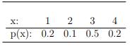
Suppose you randomly sample n = 12 observations from a discrete distribution with the following probability function:Determine E(X¯) and σ2 X¯. X: 1 2 34 p(x): 0.2 0.1 0.5 0.2
If n = 10 observations are randomly sampled from a distribution with mean µ = 9 and variance σ2 = 8, what is the mean and variance of the sample mean?
Describe the two components of a random sample.
For the following situations, (a) n = 12, σ = 22, X¯ = 65, (b) n = 22, σ = 10, X¯ = 185, (c) n = 50, σ = 30, X¯ = 19, compute a 0.95 confidence interval for the mean.
A manufacturer claims that its light bulbs have an average life span of µ = 1200 h with a standard deviation of σ = 25.If you randomly test 36 light bulbs and find that their average life span is X¯ = 1150, does a 0.95 confidence interval for µ suggest that the claim µ = 1200 is unreasonable?
Repeat the previous example, only compute a 0.99 confidence interval instead.
Assuming random sampling is from a normal distribution with standard deviationσ = 5, if you get a sample mean of X¯ = 45 based on n = 25 participants, what is the 0.95 confidence interval for µ?
If you want to compute a 0.80, 0.92, or a 0.98 confidence interval for µ when σ is known, and sampling is from a normal distribution, what values for c should you use in Equation (4.8)?
Explain the meaning of a 0.95 confidence interval.
Bayes’ theorem states the following: P(A|B) = P(B|A)P(A)/P(B). Imagine that with probability 0.9, a diagnostic test correctly identifies those individuals who have an illness, and correctly rules out a disease with probability 0.95 among individuals who do not have it. Further imagine that the
In the previous problem, determine E(X), the variance of X, E(ˆp), and the variance of ˆp.
If for a binomial, p = 0.4 and n = 25, determine (a) P(X < 11), (b) P(X ≤ 11),(c) P(X > 9), and (d) P(X ≥ 9)
The Department of Agriculture of the United States reports that 75% of all people who invest in the futures market lose money. Based on the binomial probability function, with n = 5, determine (a) the probability that all 5 lose money, (b) the probability that all 5 make money, (c) the probability
Determine P(µ − σ ≤ X ≤ µ + σ) for the probability function x: 1, 2, 3, 4 p(x): 0.2, 0.4, 0.3, 0.1
If a distribution is skewed, is it possible that the mean exceeds the 0.85 quantile?
If a distribution appears to be bell-shaped and symmetric about its mean, can we assume that the probability of being within one standard deviation of the mean is 0.68?
Showing 3100 - 3200
of 8686
First
25
26
27
28
29
30
31
32
33
34
35
36
37
38
39
Last
Step by Step Answers