New Semester
Started
Get
50% OFF
Study Help!
--h --m --s
Claim Now
Question Answers
Textbooks
Find textbooks, questions and answers
Oops, something went wrong!
Change your search query and then try again
S
Books
FREE
Study Help
Expert Questions
Accounting
General Management
Mathematics
Finance
Organizational Behaviour
Law
Physics
Operating System
Management Leadership
Sociology
Programming
Marketing
Database
Computer Network
Economics
Textbooks Solutions
Accounting
Managerial Accounting
Management Leadership
Cost Accounting
Statistics
Business Law
Corporate Finance
Finance
Economics
Auditing
Tutors
Online Tutors
Find a Tutor
Hire a Tutor
Become a Tutor
AI Tutor
AI Study Planner
NEW
Sell Books
Search
Search
Sign In
Register
study help
business
statistics informed decisions using data
Foundations Of Statistics For Data Scientists With R And Python 1st Edition Alan Agresti - Solutions
and ρ =
Inadiagnostictestforadisease,asin Section 2.1.4 let D denote theeventofhavingthe disease, andlet + denote apositivediagnosisbythetest.Letthe sensitivity π1 = P(+ S D), the false positiverate π2 = P(+ S Dc), andthe prevalence ρ = P(D). Relevanttoapatientwhohas receivedapositivediagnosisis P(D S
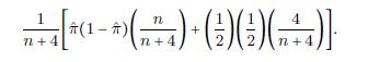
Showthatwith y successes in n binary trials,the95%scoreconfidenceinterval(4.7)for π:(a) Hasmidpoint(4.9)thatisapproximately ˜π = (y+2)~(n+4), thatis,thesampleproportion after weaddtwosuccessesandtwofailurestothedataset.(b) Hassquareofthecoefficientof zα~2 in
Bias-variancetradeoff3: For n independentweightchangesinananorexiastudy,aresearcher believesitplausiblethat μ = 0 and toestimate μ decides tousetheestimator ˜μ = cY for a constant c with 0 ≤ c ≤ 1.(a) Show that as c decreases from1to0,|bias|increasesbutvar(˜μ) decreases.(b)
Bias-variancetradeoff2: Somestatisticalmethodsdiscussedin Chapters 7 and 8 use a“shrinkage” or“smoothing”oftheMLestimator,suchthatastheamountofshrinkagein-creases, thebiasincreasesbutthevariancedecreases.Toillustratehowthiscanhappen,for Y ∼ binom(n, π), let ˜π = (Y + c)~(n + 2c)
Bias-variance tradeoff : Forabinomialparameter π, considertheBayesianestimator (Y +1)~(n + 2) that occurswithauniformpriordistribution.(a) Deriveitsbiasanditsvariance.ComparethesewiththebiasandvarianceoftheML estimator ˆπ = Y ~n.(b) ShowthatitsMSE = [nπ(1−π)+(1−2π)2]~(n+2)2. For n = 10
For n independentobservations {yi} from aPoissondistributionwithmean μ:(a) Findthescorestatistic U(y,μ) and theinformation I(μ).(b) Showhowtofindascoreconfidenceintervalfor μ.
Forthebootstrapmethod,explainthesimilarityanddifferencebetweenthetruesampling distribution of ˆθ and theempirically-generatedbootstrapdistributionintermsofitscenter and itsspread.
Suppose y1, ...,yn are independentobservationsfromaPoissondistributionwithmeanparam-eter μ. WithaBayesianapproach,weuseagamma(k,λ) priordistributionfor μ. Then,find the posteriordistributionfor μ and giveitsapproximatemeanforlarge n. (Thegammaisthe conjugate
Forabinom(n, π) observation y, considertheBayesestimatorof π using abeta(α, β) prior distribution.(a) Forlarge n, showthattheposteriordistributionof π has approximatemean ˆπ = y~n. (It also hasapproximatevariance ˆπ(1 − ˆπ)~n.) Interpret,andrelatetoclassicalinference.(b)
Refertothepreviousexercise.SupposethattheBayesian95%posteriorintervalis(23.5,25.0).Interpret,andcomparetotheproperinterpretationofaclassical95%confidenceinterval.
and25.0years.(d) Ifwerepeatedlysampledtheentirepopulation,then95%ofthetimethepopulationmean wouldbebetween23.5and25.0years.
Arandomsampleof50recordsyieldsa95%confidenceintervalforthemeanageatfirst marriage ofwomeninacertaincountyof23.5to25.0years.Explainwhatiswrongwitheach of thefollowinginterpretations.(a) Ifrandomsamplesof50recordswererepeatedlyselected,then95%ofthetimethesample mean
Let Y denote astandardCauchyrandomvariable,thatis,a t-distributed randomvariablewith df = 1.(a) Fromthedefinitionofthe t distribution in Section 4.4.5, showthat Y can beexpressed as aratiooftwoindependentstandardnormalrandomvariables.(b)
Inthe T pivotalquantityforcomparingtwomeans,explainwhy X2 = (n1 + n2 − 2)S2~σ2 has a chi-squareddistributionwith d = n1 + n2 − 2 degrees offreedom.
Usingthedefinitionofthechi-squareddistributionin Section 4.4.5, proveits reproductive property: If X2 1 and X2 2 are independentchi-squaredrandomvariableswith X2 1 ∼ χ2 d1 and X2 2 ∼ χ2 d2 , then X2 1 +X2 2 ∼ χ2 d1+d2 .
Consider n independentobservationsfromanexponential pdf f(y; λ) = λe−λy for y ≥ 0, with parameter λ > 0 for which E(Y ) = 1~λ.(a) Findthesufficient statisticforestimating λ.(b) Findthemaximumlikelihoodestimatorof λ and of E(Y ).(c) Onecanshowthat 2λ(Σi Yi) has
and8.0.(d) Ifrandomsamplesofsize1467wererepeatedlyselected,theninthelongrun95%ofthe confidence intervalsformedwouldcontainthetruevalueof μ.(e) Ifrandomsamplesofsize1467wererepeatedlyselected,theninthelongrun95%ofthe y valueswouldfall between6.8and8.0.
and8.0.(b) Wecanbe95%confidentthat μ is between6.8and8.0.(c) Inthissample,ninety-fivepercentofthevaluesof y = numberofclosefriendsarebetween
Basedonresponsesof1467subjectsinaGeneralSocialSurvey,a95%confidenceintervalforthe mean numberofclosefriendsequals(6.8,8.0).Identifywhichofthefollowinginterpretations is (are)correct,andindicatewhatiswrongwiththeothers.(a) Wecanbe95%confidentthat y is between
Selectthecorrectresponse:Otherthingsbeingequal,quadruplingthesamplesizecausesthe width ofaconfidenceintervalforapopulationmeanorproportionto(a) double,(b) halve,(c) beonequarteraswide.
Selectthecorrectresponse:Thereasonweusea zα~2 normal quantilescoreinconstructinga confidence intervalforaproportionisthat:(a) Forlargerandomsamples,thesamplingdistributionofthesampleproportionisapprox-imately normal.(b) Thepopulationdistributionisapproximatelynormal.(c)
and draw10,000randomsamplesof size 20each.Lookatthesimulatedsamplingdistributionof ˆπ, whichishighlydiscrete.Is it bell-shapedandsymmetric?UsethistohelpexplainwhytheWaldconfidenceinterval performspoorlyinthiscase.(c) When ˆπ = 0, showthattheWaldconfidenceintervalis(0,0).As π
Usesimulationoranapp,suchasthe ExploreCoverage app at www.artofstat.com/web-apps, to exploretheperformanceofconfidenceintervalsforaproportionwhen n is notverylarge and π maybenear0or1,byrepeatedlygeneratingrandomsamplesandconstructingthe confidence intervals.Takethepopulationproportion π = 0.06,
Explainthereasoningbehindthefollowingstatement:Studiesaboutmorediversepopula-tions requirelargersamplesizes.Illustrateforestimatingmeanincomeforallmedicaldoctors compared toestimatingmeanincomeforallentry-levelemployeesatMcDonald’srestaurants.
Forasimplerandomsampleof n subjects,explainwhyitisabout95%likelythatthesample proportionhaserrornomorethan 1~ºn in estimatingthepopulation proportion.(Hint: To showthis“1~ºn rule,” findtwo standard errorswhen π = 0.50, andexplainhowthiscompares to twostandarderrorsatothervaluesof π.)
Explainwhyconfidenceintervalsarenarrowerwith(a) smallerconfidencelevels,(b) larger sample sizes.
Explainwhatismeantbya pivotal quantity.
TheHardy–Weinbergformulaforthegeneticvariationofapopulationatequilibriumstatesthat with probability π of the A allele, theprobabilitiesofgenotypes(AA, Aa, aa) are (π2, 2π(1 −π), (1−π)2). Assumeamultinomialdistribution(Section 2.6.4) for n observationswithcounts(y1, y2, y3) of
Refertotheprevioustwoexercises.Considerthesellingprices(inthousandsofdollars)inthe Houses data filementionedinExercise4.31.(a) FitthenormaldistributiontothedatabyfindingtheMLestimatesof μ and σ for that distribution.(b)
Exercise2.71mentionedthatwhen Y has positivelyskeweddistributionoverthepositivereal line, statisticalanalysesoftentreat log(Y ) as havinga N(μ, σ2) distribution. Then Y has the log-normaldistribution, whichhas pdf for y > 0, f(y; μ, σ) = [1~y(º2πσ)] exp{−[log(y) − μ]2~2σ2}.(a) For n
Consider n independentobservationsfroma N(μ, σ2) distribution.(a) Focusingon μ, findthelikelihoodfunction.Showthatthelog-likelihoodfunctionisa concave,parabolicfunctionof μ. FindtheMLestimator ˆμ.(b) Considering σ2 to beknown,findtheinformationusing(i)equation(4.3),(ii)equation(4.4).
For n independentobservations {yi} from thegamma pdf (2.10), withshapeparameter k known(suchaswiththeexponentialdistributionspecialcase):(a) FindthelikelihoodfunctionandshowthattheMLestimatorof λ is ˆλ = k~Y .(b) WhatistheMLestimator of E(Y ) = k~λ?(c) Showthatthelarge-samplevarianceof ˆλ is
Exercise2.73introducedthe Paretodistribution, whichhas pdf f(y;α) = α~yα+1 for y ≥ 1 and a parameter α > 0. Astudyusesthisfamilytomodel n independentobservationsonincome.Find thelikelihoodfunctionandtheMLestimatorof α and itsasymptoticvariance.
if n = (i) 1,(ii)5,(iii) 10.Howdoestheshapeof L(λ) changeas n increases? Whataretheimplications of thenarrowinglog-likelihood?(Also,whenthelog-likelihoodisclosertoparabolic,the distribution oftheMLestimatorisclosertonormality.)(d) Findtheinformation I(λ) using
and λ =
Forindependentobservations y1, ...,yn from theexponential pdf f(y; λ) = λe−λy for y ≥ 0, for which μ = σ = 1~λ:(a) Findthelog-likelihoodfunction L(λ).(b) FindtheMLestimator ˆλof λ.(c) Suppose y = 10. Plot L(λ) − L(ˆλ) between λ =
Forindependentobservations y1, ...,yn havingthegeometricdistribution(2.1):(a) Findasufficientstatisticfor π.(b) DerivetheMLestimatorof π.
When f is acontinuous pdf with median M, forsimplerandomsamplingthesamplemedianÃM has approximatelya N(M, 1~4[f(M)]2n) sampling distribution.(a) Considersamplingfromanormalpopulation,forwhich μ = M. Usingformula(2.8),show that ˆM has asymptoticstandarderror»π~2(σ~ºn) (for π = 3.14...).(b)
Section 4.4.6 showedthat E(s2) = σ2. Forindependentsamplingfroma N(μ, σ2) distribution,ˆσ2 = [Σi(Yi−Y )2]~n is theMLestimatorand ˜σ2 = [Σi(Yi−Y )2]~(n+1) is theestimatorhaving minimum MSE.(a) Showthat ˜σ2 is anasymptoticallyunbiasedestimatorof σ2.(b) Showthat ˆσ2 is
Isthefollowingstatementtrueorfalse?If ˆθ is anunbiasedestimatorfor θ, thenforanyfunction g, g(ˆθ) is anunbiasedestimatorfor g(θ). Iftrue,explainwhy.Iffalse,giveacounter-example.
Usingsimulation,conductaninvestigationofwhetherthesamplemeanormedianisabetter estimator ofthecommonvalueforthemeanandmedianofauniformdistribution.
Take n = 100 observationsfromastandardnormaldistributionandfindthesamplemeanand median. Dothis100,000timesandplottheirestimatedsamplingdistributions.Estimatetheir mean squarederrorsaroundthecommonpopulationmeanandmedianof0.Whichseemsto
The Afterlife data fileatthebook’swebsiteshowsdatafromthe2018GeneralSocialSurvey on postlife = beliefintheafterlife(1 = yes,2 = no) andreligion(1 = Protestant,2 = Catholic, 3 =Jewish, othercategoriesexcluded).Analyzethesedatawithmethodsofthischapter.Summarize results
The Houses data fileatthebook’swebsitelists,for100homesalesinGainesville,Florida, severalvariables,includingthesellingpriceinthousandsofdollarsandwhetherthehouse is new(1 = yes,0 = no). Prepareashortreportinwhich,statingallassumptionsincluding the
Whena2015PewResearchsurvey(www.pewresearch.org) asked Americans whetherthereis solid evidenceofglobalwarming,92%ofDemocratswhoidentifiedthemselvesasliberalsaid yes whereas 38%ofRepublicanswhoidentifiedthemselvesasconservativesaid yes. Suppose n = 200 for
Astudythat Section 7.3.2 discusses aboutendometrialcanceranalyzedhowahistologygrade responsevariable(HG = 0, low;HG = 1, high)relatestothreeriskfactors,includingNV =neovasculation(1 = present,0 = absent).Usingthe Endometrial data fileatthebook’swebsite, conduct
Refertothepreviousexercise.ConductBayesianmethodswithimproperpriorstoobtain a posteriorintervalforthepopulationmeanweightchangeforthefamilytherapyandthe difference betweenthepopulationmeansforthattherapyandthecontrolcondition.Forthe difference,
RefertoExercise4.13.ConsiderBayesianinferenceforthepopulationmeanweightchange μfor thefamilytherapy.(a) Selectdiffusepriordistributionsfor μ and σ2 and findtheposteriormeanestimateand a 95%posteriorintervalfor μ.(b) Constructtheclassical95%confidenceintervalfor μ.
Refertotheclinicaltrialexamplein Section 4.7.5. UsingtheJeffreyspriorfor π1 and for π2, simulateandplottheposteriordistributionof π1 −π2. FindtheHPDinterval.Whatdoesthat intervalreflectabouttheposteriordistribution?
Refertothepreviousexercise,regardingestimating π when y = 0 in n = 25 trials.(a) Withuniformpriordistribution,findthe95%highestposteriordensity(HPD)interval, and comparewiththe95%equal-tailposteriorinterval,usingthe2.5and97.5percentiles.Whyaretheydifferent?(b) When y = 0,
RefertothevegetariansurveyresultinExercise4.6,with n = 25 and novegetarians.(a) FindtheBayesianestimateof π using abetapriordistributionwith α = β equal (i) 0.5,(ii) 1.0,(iii) 10.0.Explainhowthechoiceofpriordistributionaffectstheposteriormean estimate.(b)
Youwanttoestimate the proportionofstudentsatyourschoolwhoanswer yes when asked whether governmentsshoulddomoretoaddressglobalwarming.Inarandomsampleof10 students,everystudentsays yes. Giveapointestimateoftheprobabilitythatthenextstudent interviewedwillanswer yes, ifyouuse(a) MLestimation,(b)
Ina2016PewResearchsurvey(www.pewresearch.org), the percentagewhofavoredallowing gaysandlesbianstomarrylegallywas84%forliberalDemocratsand24%forconservative Republicans. Suppose n = 300 for eachgroup.Usinguniformpriordistributions,(a) Construct95%posteriorintervalsforthepopulationproportions.(b)
The trimmedmean calculates thesamplemeanafterexcludingasmallpercentageofthe lowestandhighestdatapoints,tolessentheimpactofoutliers.Forexample,withthefunction mean(y, 0.05) applied toavariable y, R finds the 10% trimmedmean, excluding5%ateach end.
Toillustratehowsamplingdistributionofthecorrelationcanbehighlyskewedwhenthe the truecorrelationisnear −1 or+1,constructandplotthebootstrapdistributionforthe correlation between GDP and CO2 for the UN data. (Thisismerelyforillustration,because this datasetisnotarandomsampleofnations).
Withthedataonthenumberofyearssinceabookwascheckedout(variable C) inthe Library data fileatthetextwebsite,usethebootstraptofindandinterpretthe95% (a) percentile confidence intervalforthemedian, (b) percentileandbias-correctedconfidenceintervalsfor the standarddeviation.
Astandardizedvariable Y dealing withafinancialoutcomeisconsideredtotakeanunusually extreme valueif y > 3. Find P(Y > 3) if (a) Y is modeledashavingastandardnormaldistri-bution Y ∼ N(0, 1), (b) Y instead behaveslikearatioofstandardnormalrandomvariables, in whichcase Y has
Randomlygenerate10,000observationsfroma t distribution with df = 3 and constructa normal quantileplot(Exercise2.67).Howdoesthisplotrevealnon-normalityofthedataina waythatahistogramdoesnot?
The Substance data fileatthebook’swebsiteshowsacontingencytableformedfromasurvey that askedasampleofhighschoolstudentswhethertheyhaveeverusedalcohol,cigarettes, and marijuana.Constructa95%Waldconfidenceintervaltocomparethosewhohaveusedor not usedalcoholonwhethertheyhaveusedmarijuana,using(a)
Inthe2018GeneralSocialSurvey,whenaskedwhethertheybelievedinlifeafterdeath,1017 of 1178femalessaid yes, and703of945malessaid yes. Construct95%confidenceintervals for thepopulationproportionsoffemalesandmalesthatbelieveinlifeafterdeathandforthe difference betweenthem.Interpret.
Usingthe Students data file,forthecorrespondingpopulation,constructa95%confidencein-terval(a) forthemeanweeklynumberofhoursspentwatchingTV;(b) tocomparefemalesand males onthemeanweeklynumberofhoursspentwatchingTV.Ineachcase,stateassumptions, including
Sections 4.4.3 and 4.5.3 analyzed datafromastudyaboutanorexia.The Anorexia data file at thetextwebsitecontainsresultsforthecognitivebehavioralandfamilytherapiesandthe controlgroup.Usingdataforthe17girlswhoreceivedthefamilytherapy:(a)
The Income data fileatthebook’swebsiteshowsannualincomesinthousandsofdollarsfor subjectsinthreeracial-ethnicgroupsintheU.S.(a) Useagraphicsuchasaside-by-sideboxplot(Section 1.4.5) tocompareincomesofBlack, Hispanic, andWhitesubjects.(b)
TheobservationsonnumberofhoursofdailyTVwatchingforthe10subjectsinthe2018GSS who identifiedthemselvesasIslamicwere0,0,1,1,1,2,2,3,3,4.(a) Constructandinterpreta95%confidenceintervalforthepopulationmean.(b) Supposetheobservationof4wasincorrectlyrecordedas24.Whatwouldyouobtainfor the
ArecentGeneralSocialSurveyaskedmalerespondentshowmanyfemalepartnerstheyhave had sexwithsincetheir18thbirthday.Forthe131malesbetweentheagesof23and29,the median = 6 andmode = 1 (16.8%ofthesample).Softwaresummarizesotherresults:Variable nMeanStDevSEMean95.0%CI NUMWOMEN
Astudyinvestigatesthedistributionofannualincomeforheadsofhouseholdslivinginpublic housing inChicago.Forarandomsampleofsize30,theannualincomes(inthousandsof dollars) areinthe Chicago data fileatthetextwebsite.(a) Basedonadescriptivegraphic,describetheshapeofthesampledatadistribution.Find and
ToestimatetheproportionoftrafficdeathsinCalifornialastyearthatwerealcoholrelated,de-termine thenecessarysamplesizefortheestimatetobeaccuratetowithin0.04withprobability 0.90. BasedonresultsofstudiesreportedbytheNationalHighwayTrafficSafetyAdministra-tion (www.nhtsa.gov), we
AsocialscientistwantedtoestimatetheproportionofschoolchildreninBostonwholivein a single-parentfamily.Shedecidedtouseasamplesizesuchthat,withprobability0.95,the error wouldnotexceed0.05.Howlargeasamplesizeshouldsheuse,ifshehasnoideaofthe size ofthatproportion?
Inarandomsampleof25people to estimatetheextentofvegetarianisminasociety,0peo-ple werevegetarian.Constructa99%Waldconfidenceintervalforthepopulationproportion of vegetarians.Explaintheawkwardissueindoingthis,andfindandinterpretamorereli-able confidenceinterval.(As Section 4.3.3
TheGeneralSocialSurveyhasaskedrespondents,“Doyouthinktheuseofmarijuanashould bemadelegalornot?”Viewresultsatthemostrecentcumulativedatafileat sda.berkeley.edu/archive.htm byenteringthevariablesGRASSandYEAR.(a) Describeanytrendyouseesince1973inthepercentagefavoringlegalization.(b)
Forthe Students data file(Exercise1.2in Chapter 1) andcorrespondingpopulation,findthe ML estimateofthepopulationproportionbelievinginlifeafterdeath.ConstructaWald95%confidence interval,usingitsformula(4.8).Interpret.
with y = 6 for n = 10 (e.g.,in R bytaking pi (π) asasequencebetween0 and 1andthentakingLasthelogof dbinom(6, 10,pi)). Identify ˆπ in theplotandexplain whymaximizationoccursatthesamepointasintheplotof ℓ(π) itself.
Plotthelog-likelihoodfunction L(π) correspondingtothebinomiallikelihoodfunction ℓ(π)shownin Figure
Forasequenceofobservationsofabinaryrandomvariable,youobservethegeometricrandom variable(Section 2.2.2) outcomeofthefirstsuccessonobservationnumber y = 3. Findandplot the likelihoodfunction.
Forapoint estimate ofthemeanofapopulationthatisassumedtohaveanormaldistribution, a datascientistdecidestousetheaverageofthesamplelowerandupperquartilesforthe n = 100 observations,sinceunlikethesamplemean ¯ Y , thequartilesarenotaffectedbyoutliers.Evaluate the precisionofthisestimatorcomparedto ¯
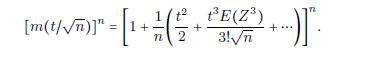
RefertoExercise3.45andthe mgf m(t) = eμt+σ2t2~2 for anormaldistribution.For n indepen-dentobservations {Yi} from anarbitrarydistributionwithmean μ and variance σ2, let m(t)bethe mgf of thestandardizedrandomvariable Zi = (Yi − μ)~σ.(a) Explainwhythe mgf of ºn(Y − μ)~σ is [m(t~ºn)]n.(b)
RefertoExercise2.66and the momentgeneratingfunction m(t) = EetY , analternativeto the probabilityfunctionforcharacterizingaprobabilitydistribution.Forindependentrandom variables Y1, Y2, …, Yn, let T = Y1 + ⋯+ Yn.(a) Explainwhy T has mgf determined bytheseparateonesas m(t) =
and π2 = 0.10. Simulateamillionsample proportionsfromeachtreatmentwith n1 = n2 = 50. Constructhistogramsfor ˆπ1~ˆπ2 and for log(ˆπ1~ˆπ2). Whichseemstohavesamplingdistributionclosertonormality?(This showsthatsomestatisticsmayrequireaverylargesamplesizetohaveanapproximate normal
Forindependent Y1 ∼ binom(n1, π1) and Y2 ∼ binom(n2, π2) random variables, ˆπ1~ˆπ2 is called the relativerisk or risk ratio. Thismeasureisoftenusedinmedicalresearchtocomparethe probabilityofacertainoutcomefortwotreatments.(a) Arandomizedstudywith n1 = n2 = 50 compares
When T is astandard normal randomvariable,whydoesthedeltamethodnotimplythat T2 has anormaldistribution?(Hint: FormtheTaylor-seriesexpansionof g(t) = t2 around g(0).In Section 4.4.5 weshallseethat T2 has achi-squareddistribution.)
Manypositively-valuedresponsevariableshaveaunimodaldistributionbutwithstandard deviation proportionaltothemean.Identifyatransformationforwhichthevarianceisapprox-imately thesameforallvaluesofthemean.Identifyatleastonedistributionthathasstandard deviation proportionaltothemean.
Forabinomialsample proportion ˆπ, showthattheapproximatevarianceof sin−1(ºˆπ) (with the anglebeingmeasured in radians)is1/4n, sothisisavariancestabilizingtransformation.(In reality,simulationrevealsthatthevarianceofthis arcsinetransformation is notnearly constantwhen π is near0ornear1and n
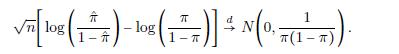
Forabinomialparameter π, g(π) = log[π~(1 − π)] is calledthe logit. Itisusedforcategorical data, asshownin Chapter 7. Let T = ˆπ for n independentbinarytrials.Usethedeltamethod to showthat Vlog()()(0-1)). villog()-10g( N
Explainthedifferencebetween convergenceinprobability and convergenceindistribution.Explain howonecanregardconvergenceinprobabilityasaspecialcaseofconvergencein distribution forwhichthelimitingdistributionhasprobability1atasinglepoint.
is reasonableforgivingabellshape.Forthis M, showthat Y has anapproximatenormal sampling distributionwhen n ≥ 10S2. Forthis guideline, howlargearandomsampledoyouneedfromanexponentialdistributionto achieveclosetonormalityforthesamplingdistribution?
Consider n independentobservationsofarandomvariable Y that hasskewnesscoefficient S = E(Y − μ)3~σ3.(a) Showhow E(Y −μ)3 relates to E(Y −μ)3. Based on this,showthattheskewnesscoefficient for thesamplingdistributionof Y satisfies skewness(Y ) = S~ºn. Explainhowthis result relates
Theformula σY= σ~ºn for thestandarderrorof Y treats thepopulation size as infinitely large relativetothesamplesize n. Withafinitepopulationsize N, separateobservationsare veryslightlynegativelycorrelated,sovar(Σi Yi) < Σivar(Yi), andactuallyThe term »(N − n)~(N − 1) is calledthe finite
Forindependentobservations,var(Σi Yi) = Σi var(Yi). Explainintuitivelywhy Σi Yi has a larger variancethanasingleobservation Yi.
Inthepreviousexercise,explainwhatisincorrectabouteachoptionthatyoudidnotchoose.
TheCentralLimitTheoremimpliesthat(a) Allvariableshaveapproximatelybell-shapedsampledatadistributionsifarandomsample containsatleastabout30observations.(b) Populationdistributionsarenormalwheneverthepopulationsizeislarge.(c) Forlarge random samples,thesamplingdistributionof Y is
Inonemilliontossesofafaircoin,theprobabilityofgettingexactly500,000headsand500,000 tails (i.e.,asampleproportionofheadsexactly=1/2)is(a) verycloseto1.0,bythelawoflargenumbers.(b) verycloseto1/2,bythelawoflargenumbers.(c) verycloseto0,bythestandarddeviationofthebinomialdistributionanditsapproximate
Thestandarderrorofastatisticdescribes(a) Thestandarddeviationofthesamplingdistributionofthatstatistic.(b) Thestandarddeviationofthesampledata.(c) Howclosethatstatisticislikelytofalltotheparameterthatitestimates.(d) Thevariabilityinvaluesofthestatisticforrepeatedsimplerandomsamplesofsize n.(e)
Whichdistributiondoesthesampledatadistributiontendtoresemblemoreclosely—thesam-pling distributionofthesamplemeanorthepopulationdistribution?Explain.Illustrateyour answerforavariable Y that
and σ = 7.75. Plot the populationdistributionandthesimulatedsamplingdistributionofthe10,000 y values.Explain whatyour plotsillustrate.
bytaking10,000simulations of arandomsampleofsize n = 200 from agammadistributionwith μ =
MimictheappdisplayoftheCentralLimitTheoremin Figure
and amedianof0.69.As n increases, doesthesamplingdistributionofthesamplemedianseemtobeapproximately normal?
Simulatefor n = 10 and n = 100 the samplingdistributionsofthesamplemedianforsampling from theexponentialdistribution(2.12)with λ = 1.0, whichhas μ = σ =
Asurveyisplannedtoestimatethepopulationproportion π supportingmoregovernment action toaddressglobalwarming.Forasimplerandomsample,if π maybenear0.50,how large should n besothatthestandarderrorofthesampleproportionis0.04?
Showing 2700 - 2800
of 5564
First
21
22
23
24
25
26
27
28
29
30
31
32
33
34
35
Last
Step by Step Answers