New Semester
Started
Get
50% OFF
Study Help!
--h --m --s
Claim Now
Question Answers
Textbooks
Find textbooks, questions and answers
Oops, something went wrong!
Change your search query and then try again
S
Books
FREE
Study Help
Expert Questions
Accounting
General Management
Mathematics
Finance
Organizational Behaviour
Law
Physics
Operating System
Management Leadership
Sociology
Programming
Marketing
Database
Computer Network
Economics
Textbooks Solutions
Accounting
Managerial Accounting
Management Leadership
Cost Accounting
Statistics
Business Law
Corporate Finance
Finance
Economics
Auditing
Tutors
Online Tutors
Find a Tutor
Hire a Tutor
Become a Tutor
AI Tutor
AI Study Planner
NEW
Sell Books
Search
Search
Sign In
Register
study help
computer science
digital control system analysis and design
Digital Signal Processing System Analysis And Design 2nd Edition Paulo S. R. Diniz, Eduardo A. B. Da Silva , Sergio L. Netto - Solutions
Design a linear-phase lapped biorthogonal transform with \(M=10\) sub-bands.
Design a length-16 linear-phase lapped biorthogonal transform with \(M=8\) sub-bands aiming at minimizing the stopband ripple of the sub-filters.
Design a GenLOT with \(M=10\) sub-bands having at least \(25 \mathrm{~dB}\) of stopband attenuation.
Design a GenLOT with \(M=8\) sub-bands having at least \(25 \mathrm{~dB}\) of stopband attenuation.
Design a GenLOT with \(M=6\) sub-bands having at least \(20 \mathrm{~dB}\) of stopband attenuation.
Show that if a filter bank has linear-phase analysis and synthesis filters with the same lengths \(N=L M\), then the following relations for the polyphase matrices are valid:\[\begin{aligned}& \mathbf{E}(z)=z^{-L+1} \mathbf{D E}\left(z^{-1}\right) \mathbf{J} \\& \mathbf{R}(z)=z^{-L+1} \mathbf{J
Consider an \(M\)-band linear-phase filter bank with perfect reconstruction with all analysis and synthesis filters having the same length \(N=L M\). Show that, for a polyphase matrix \(\mathbf{E}_{1}(z)\) corresponding to a linear-phase filter bank, then \(\mathbf{E}(z)=\mathbf{E}_{2}(z)
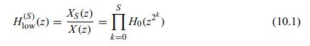
Deduce Equations (10.1)-(10.4). (S) low (2) How S = Xs(z) X(z) =Ho (22) (10.1) k=0
Consider a two-band linear-phase filter bank whose product filter \(P(z)=\) \(H_{0}(z) H_{1}(-z)\) of order \((4 M-2)\) can be expressed as\[P(z)=z^{-2 M+1}+\sum_{k=0}^{M-1} a_{2 k}\left(z^{-2 k}+z^{-4 M+2+2 k}\right)\]Show that such a \(P(z)\) :(a) Can have at most \(2 M\) zeros at \(z=-1\).(b)
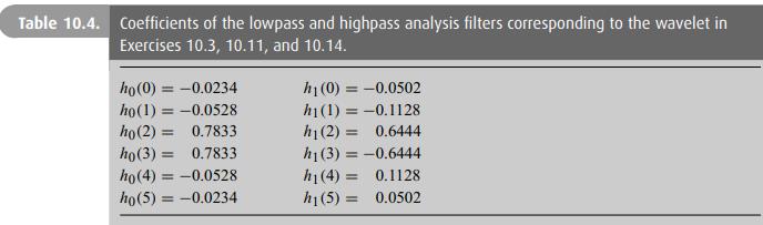
Compute the analysis and synthesis wavelets and scaling functions corresponding to the analysis filters in Table 10.4. Table 10.4. Coefficients of the lowpass and highpass analysis filters corresponding to the wavelet in Exercises 10.3, 10.11, and 10.14. ho(0) = -0.0234 ho(1) = -0.0528 ho(2)=0.7833
Show that the sub-bands from a two-band decomposition of a periodic signal with odd period \(N\) have \(2 N\) independent samples.
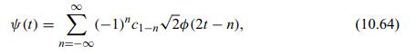
Show that \(\psi(t)\) as defined in Equation (10.64) is orthogonal to \(\phi(t-n)\) and that \(\psi(t-n)\), for \(n \in \mathbb{Z}\), is an orthonormal basis for \(W_{0}\) (Vetterli \& Kovačević, 1995; Mallat, 1999). (t)=(-1)" c-n20 (21-n), 11=- (10.64)
For a two-band perfect reconstruction filter bank, assume the analysis filter \(H_{0}(z)\) and the synthesis filter \(G_{0}(z)\) satisfy the condition of Equation (10.142). Assume also that these filters were designed to generate a wavelet so that they have enough zeros placed at \(z=1\).(a) Show
Apply the technique, known as balancing, described in Exercise 10.6, to the filters of Equations (10.204) and (10.205) and comment on the observed results.Exercise 10.6,For a two-band perfect reconstruction filter bank, assume the analysis filter \(H_{0}(z)\) and the synthesis filter \(G_{0}(z)\)
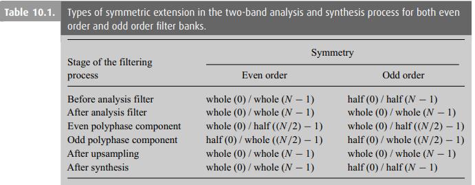
Develop a table similar to Table 10.1 for computing symmetric extensions of oddlength signals. Note in this case that for odd order the lowpass and highpass bands may not have the same lengths. Table 10.1. Types of symmetric extension in the two-band analysis and synthesis process for both even
Quantization of wavelet transforms: use the signal generated in Experiment 10.1 and compute its \(N\)-stage wavelet transform with both the bior 4.4 and the \(\mathrm{db} 4\) wavelets. Use \(N=3, N=6\), and \(N=8\). Quantize its coefficients using several quantization step sizes \(q\). Use for the
Repeat Exercise 10.9, this time using as input the image cameraman. tif from the MATLAB Image Processing Toolbox. Observe how the increase in the quantization step sizes affects the reconstructed image quality.Exercise 10.9, Quantization of wavelet transforms: use the signal generated in
Repeat Exercise 10.10 using the filter bank whose analysis lowpass and highpass filters are listed in Table 10.4. Compare the results with those obtained in Exercise 10.10 for the same quantization step sizes.Exercise 10.10Repeat Exercise 10.9, this time using as input the image cameraman. tif
Repeat Exercises 10.10 and 10.11, this time comparing the results obtained from the use of the periodic and symmetric extensions. Refer to the MatLab function dwtmode, which sets the type of signal extension used when computing wavelet transforms.Exercise 10.11Repeat Exercise 10.10 using the filter
Compute the number of vanishing moments of the analysis and synthesis wavelets of Exercise 10.3, using, for instance, the MATLAB function \(t f 2 \mathrm{zp}\).Exercise 10.3,Compute the analysis and synthesis wavelets and scaling functions corresponding to the analysis filters in Table 10.4. Table
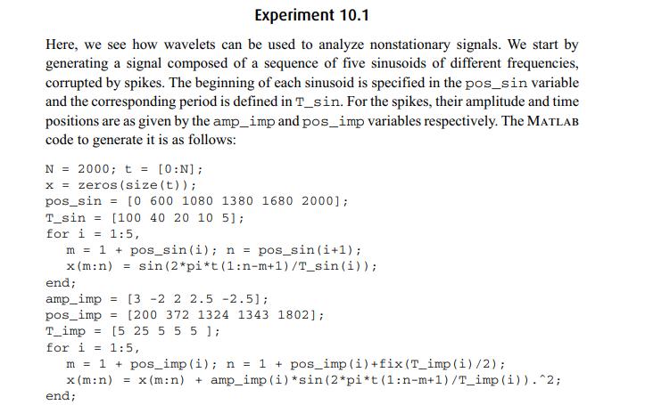
Compute the STFT of the signal generated in Experiment 10.1 and compare it with the wavelet transform obtained in Experiment 10.1, using the MATLAB command spectrogram. Describe the differences in the representations of sinusoids and impulses in both cases. Experiment 10.1 Here, we see how wavelets
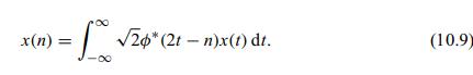
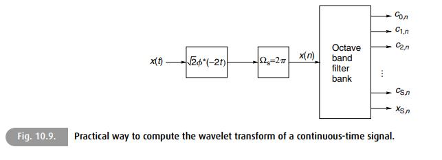
If one wants to compute the wavelet transform of a continuous signal, then one has to assume that its digital representation is derived as in Equation (10.9) and Figure 10.9. However, the digital representation of a signal is usually obtained by filtering it with a band-limiting filter and sampling
Design a circuit that determines the two's complement of a binary number in a serial fashion.
Show, using Equation (11.20), that, if \(X\) and \(Y\) are represented in two's-complement arithmetic, then:(a) \(X-Y=X+c[Y]\), where \(c[Y]\) is the two's complement of \(Y\).(b) \(X-Y=\overline{Y+\bar{X}}\), where \(\bar{X}\) represents the number obtained by inverting all bits of \(X\).
Describe an architecture for the parallel multiplier where the coefficients are represented in the two's-complement format.
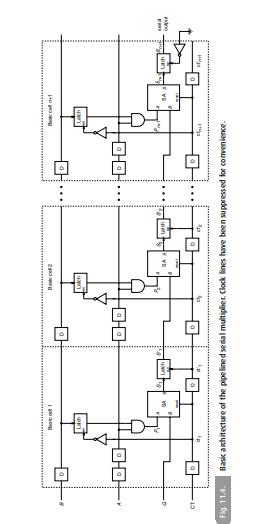
Describe the internal circuitry of the multiplier in Figure 11.4 for 2-bit input data. Then perform the multiplication of several combinations of data, determining the internal data obtained at each step of the multiplication operation. CT Fig.11.4. Ladh 2 SA With chit Basic architecture of
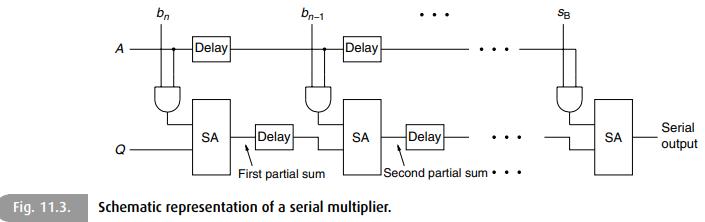
Describe the implementation of the FIR digital filter in Figure 4.3 using the distributed arithmetic technique. Design the architecture in detail, specifying the dimensions of the memory unit as a function of the filter order. bn Delay bn-1 Delay SB Serial SA Delay SA Delay SA output First partial
Determine the content of the memory unit in a distributed arithmetic implementation of the direct-form realization of a digital filter whose coefficients are given by\[\begin{aligned}& b_{0}=b_{2}=0.07864 \\& b_{1}=-0.14858 \\& a_{1}=-1.93683 \\& a_{2}=0.95189 .\end{aligned}\]Use 8 bits to
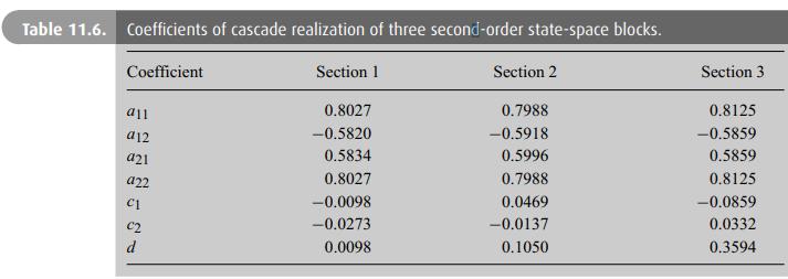
Determine the content of the memory unit in a distributed arithmetic implementation of the cascade realization of three second-order state-space blocks whose coefficients are given in Table 11.6 (scaling factor: \(\lambda=0.2832\) ). Table 11.6. Coefficients of cascade realization of three
Describe the number -0.832645 using one's-complement, two's-complement, and CSD formats.
Describe the number -0.00061245 in floating-point representation, with the mantissa in two's complement.
Deduce the probability density function of the quantization error for the signmagnitude and one's-complement representations. Consider the cases of rounding, truncation, and magnitude truncation.
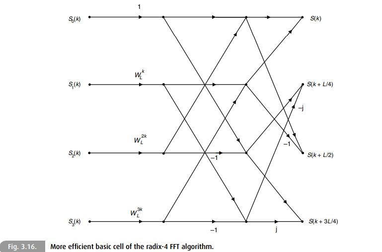
Calculate the scaling factors for the radix-4 butterfly of Figure 3.16 using the \(L_{2}\) and \(L_{\infty}\) norms. So(K) S(K) S(K) W S(k + L/4) S(K) 2k W 3k W S(K) -1 Fig. 3.16. More efficient basic cell of the radix-4 FFT algorithm. S(k + L/2) S(k + 3L/4)
Show that the \(L_{2}\) norm of the transfer function\[H(z)=\frac{b_{1} z+b_{2}}{z^{2}+a_{1} z+a_{2}}\]is\[\|H(z)\|_{2}^{2}=\frac{\left(b_{1}^{2}+b_{2}^{2}\right)\left(1+a_{2}\right)-2 b_{1} b_{2} a_{1}}{\left(1-a_{1}^{2}+a_{2}^{2}+2 a_{2}\right)\left(1-a_{2}\right)} .\]
Given the transfer function\[H(z)=\frac{1-\left(a z^{-1}\right)^{M+1}}{1-a z^{-1}}\]compute the scaling factors using the \(L_{2}\) and \(L_{\infty}\) norms assuming \(|a|
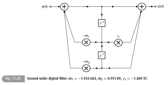
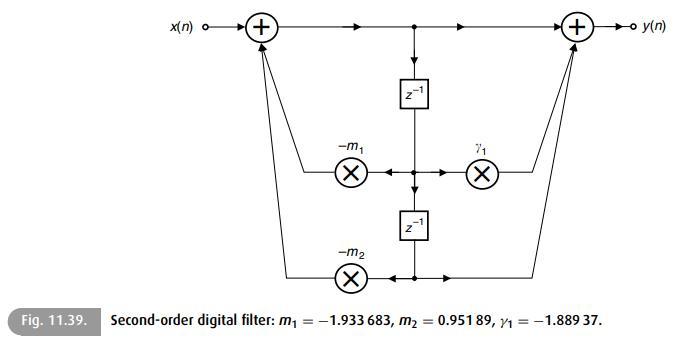
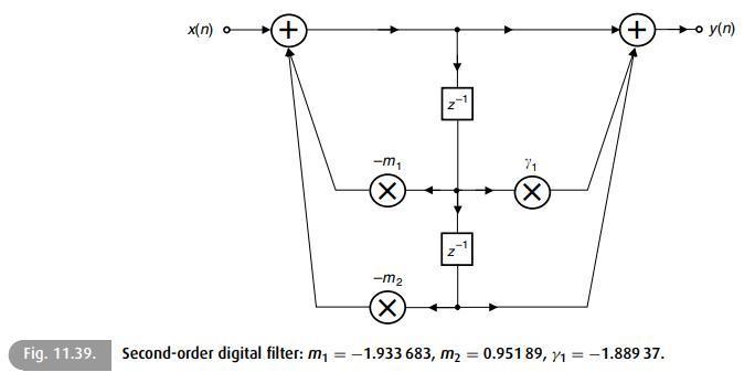
Calculate the scaling factor for the digital filter in Figure 11.39, using the \(L_{2}\) and \(L_{\infty}\) norms. Fig. 11.39. x(n) o + -m (X) ( + -o y(n) -m2 () Second-order digital filter: m = -1.933 683, m = 0.951 89, 1 = -1.889 37.
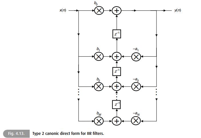
Show that, for the Type 2 canonic direct-form realization for IIR filters (as depicted in Figure 4.13), the scaling coefficient is given by\[\lambda=\frac{1}{\max \left\{1,\|H(z)\|_{p}\right\}}\]Figure 4.13 b x(n) (X) (+) y(n) -a +) ( -22 (X) + ( -an bM + (X) Fig. 4.13. Type 2 canonic direct form
Calculate the relative output-noise variance in decibels for the filter of Figure 11.39 using fixed-point and floating-point arithmetics. Fig. 11.39. x(n) o + -m (X) ( + -o y(n) -m2 (X) Second-order digital filter: m = -1.933 683, m = 0.951 89, 1=-1.889 37.
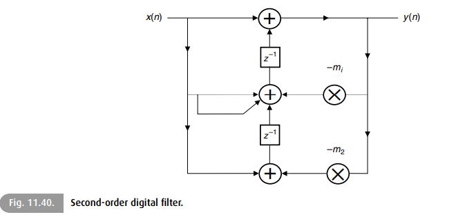
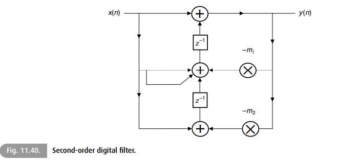
Calculate the output-noise RPSD for the filter in Figure 11.40 using fixed-point and floating-point arithmetics. x(n) + + -mi (X -m2 + (X Fig. 11.40. Second-order digital filter. y(n)
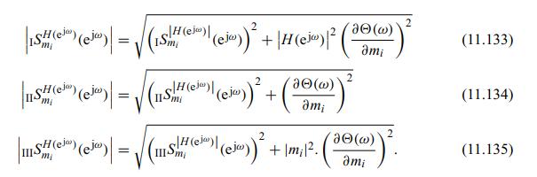
Derive Equations (11.133)-(11.135). ISH (e) 'mi = 2 SH (ei) | (ejo)) + |H (ejo) | ( 2 a(w) (11.133) mi |H(ej)| a(w) = (ej + (11.134) mi ami 2 = mi mi *+ m (30) 2 (11.135) ami
Calculate the maximum expected value of the transfer function deviation, given by the maximum value of the tolerance function, with a confidence factor of \(95 \%\), for the digital filter in Figure 11.39 implemented with 6 bits. Use \(H\left(\mathrm{e}^{\mathrm{j}
Determine the minimum number of bits a multiplier should have to keep a signalto-noise ratio above \(80 \mathrm{~dB}\) at its output. Consider that the type of quantization is rounding.
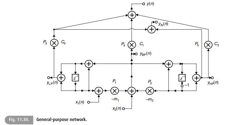
Plot the pole grid for the structure of Figure 11.30 when the coefficients are implemented in two's complement with 6 bits, including the sign bit. Fig. 11.30. P3 Co + 0+ (+ YLP(n) + -o y(n) YN(n) + P X G O YBP(n) P P (X) + (X) -m -m2 x(n) X(n) o General-purpose network. P5 (X) C + (+ ()
Discuss whether granular limit cycles can be eliminated in the filter of Figure 11.40 by using magnitude truncation quantizers at the state variables. x(n) + -mi + (X) -m2 + (X) Fig. 11.40. Second-order digital filter. y(n)
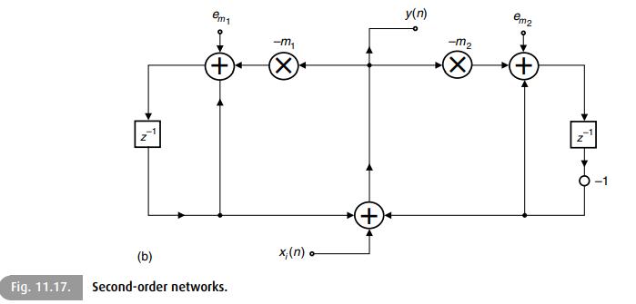
Verify whether it is possible to eliminate granular and overflow limit cycles in the structure of Figure 11.17b. em (+ -m (X y(n) -m2 ( em2 + (b) Fig. 11.17. Second-order networks. x;(n) +
Plot the overflow characteristics of simple one's-complement arithmetic.
Suppose there is a structure that is free from zero-input limit cycles, when employing magnitude truncation, and that it is also forced-input stable when using saturation arithmetic. Discuss whether overflow oscillations occur when the overflow quantization is removed, with the numbers represented
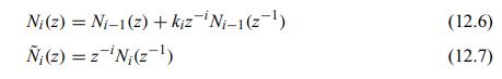
Prove Equations (12.6) and (12.7). Ni(z) = Ni-1(2) + kiz'Ni-1 (z) (12.6) (z) = z Ni(z) (12.7)
Write down a MatLab command that determines the FIR lattice coefficients from the FIR direct-form coefficients.
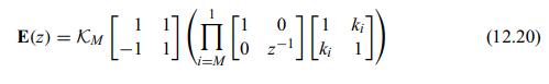
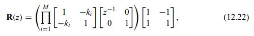
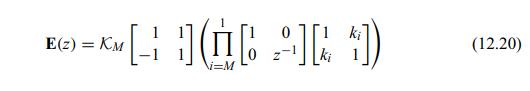
For \(\mathbf{E}(z)\) and \(\mathbf{R}(z)\) defined as in Equations (12.20) and (12.22), show that:(a) \(\mathbf{E}(z) \mathbf{R}(z)=z^{-M}\).(b) The synthesis filter bank has linear phase. E(z) = KM 9-(99) (12.20) i=M
Synthesize a two-band lattice filter bank for the case such that\[H_{0}(z)=z^{-5}+2 z^{-4}+4 z^{-3}+4 z^{-2}+2 z^{-1}+1 .\]Determine the corresponding \(H_{1}(z)\).
Design a two-band QMF filter bank satisfying the following specifications:\[\begin{aligned}\delta_{\mathrm{p}} & =0.5 \mathrm{~dB} \\\delta_{\mathrm{r}} & =40 \mathrm{~dB} \\\Omega_{\mathrm{p}} & =0.45 \frac{\Omega_{\mathrm{s}}}{2} \\\Omega_{\mathrm{r}} & =0.55 \frac{\Omega_{\mathrm{s}}}{2}
Design a two-band perfect-reconstruction filter bank with linear-phase subfilters satisfying the following specifications:\[\begin{aligned}\delta_{\mathrm{p}} & =1 \mathrm{~dB} \\\delta_{\mathrm{r}} & =60 \mathrm{~dB} \\\Omega_{\mathrm{p}} & =0.40 \frac{\Omega_{\mathrm{s}}}{2} \\\Omega_{\mathrm{r}}
A lattice-like realization with second-order section allows the design of linear-phase two-band filter banks with even order where both \(H_{0}(z)\) and \(H_{1}(z)\) are symmetric. In this case\[\mathbf{E}(z)=\left(\begin{array}{cc}\alpha_{1} & 0 \\0 &
Design a highpass filter using the minimax method satisfying the following specifications:\[\begin{aligned}A_{\mathrm{p}} & =0.8 \mathrm{~dB} \\A_{\mathrm{r}} & =40 \mathrm{~dB} \\\Omega_{\mathrm{r}} & =5000 \mathrm{~Hz} \\\Omega_{\mathrm{p}} & =5200 \mathrm{~Hz} \\\Omega_{\mathrm{s}} & =12000
Use the MATLAB commands filter and filt latt with the coefficients obtained in Exercise 12.9 to filter a given input signal. Verify that the output signals are identical. Compare the processing time and the total number of floating-point operations used by each command, using tic, toc, and
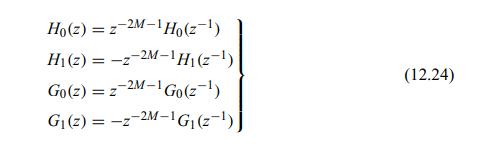
Show that the linear-phase relations in Equation (12.24) hold for the analysis filters when their polyphase components are given by Equation (12.20). Ho(z) =z-2M-1 Ho(z) H(2)=-2-2M-H(2-1) Go(z) =z-2M-1 Go (z-) G(z) = -z-2M-1 G(z) (12.24)
Use the MATLAB commands \(\mathrm{filt} \mathrm{ter}\), conv, and \(\mathrm{f} f \mathrm{t}\) to filter a given input signal, with the impulse response obtained in Exercise 12.9. Verify what must be done to the input signal in each case to force all output signals to be identical. Compare the
Discuss the distinct feature of an RRS filter with even and odd values of \(M\).
By replacing \(z\) with \(-z\) in an RRS filter, where will its pole and zeros be located? What type of magnitude response will result?
Replace \(z\) by \(z^{2}\) in an RRS filter and discuss the properties of the resulting filter.
Plot the magnitude response of the modified-sinc filter with \(M=2,4,6,8\). Choose an appropriate \(\omega_{0}\) and compare the resulting passband widths.
Plot the magnitude response of the modified-sinc filter with \(M=7\). Choose four values for \(\omega_{0}\) and discuss the effect on the magnitude response.
Given the transfer function below\[H(z)=-z^{-2 N}+\cdots-z^{-6}+z^{-4}-z^{-2}+1\]where \(M\) is an odd number:(a) Show a realization with the minimum number of adders.(b) For a fixed-point implementation, determine the scaling factors of the filter for the \(L_{2}\) and \(L_{\infty}\) norms.(c)
Design a lowpass filter using the prefilter and interpolation methods satisfying the following specifications:\[\begin{aligned}A_{\mathrm{p}} & =0.8 \mathrm{~dB} \\A_{\mathrm{r}} & =40 \mathrm{~dB} \\\Omega_{\mathrm{p}} & =4500 \mathrm{~Hz} \\\Omega_{\mathrm{r}} & =5200 \mathrm{~Hz}
Repeat Exercise 12.19 using the modified-sinc structure as building block.Exercise 12.19 Design a lowpass filter using the prefilter and interpolation methods satisfying the following specifications:\[\begin{aligned}A_{\mathrm{p}} & =0.8 \mathrm{~dB} \\A_{\mathrm{r}} & =40 \mathrm{~dB}
Demonstrate quantitatively that FIR filters based on the prefilter and the interpolation methods have lower sensitivity and reduced output roundoff noise than the minimax filters implemented using the direct form, when they satisfy the same specifications.
Design a lowpass filter using the frequency-response masking method satisfying the following specifications:\[\begin{aligned}A_{\mathrm{p}} & =2.0 \mathrm{~dB} \\A_{\mathrm{r}} & =40 \mathrm{~dB} \\\omega_{\mathrm{p}} & =0.33 \pi \mathrm{rad} / \mathrm{sample} \\\omega_{\mathrm{r}} & =0.35 \pi
Design a highpass filter using the frequency-response masking method satisfying the specifications in Exercise 12.9. Compare the results obtained with and without an efficient ripple margin distribution, with respect to the total number of multiplications per output sample, with the results
Design a bandpass filter using the quadrature method satisfying the following specifications:\[\begin{aligned}A_{\mathrm{p}} & =0.02 \mathrm{~dB} \\A_{\mathrm{r}} & =40 \mathrm{~dB} \\\Omega_{\mathrm{r}_{1}} & =0.068 \pi \mathrm{rad} / \mathrm{s} \\\Omega_{\mathrm{p}_{1}} & =0.07 \pi \mathrm{rad} /
Design a bandstop filter using the quadrature method satisfying the following specifications:\[\begin{aligned}A_{\mathrm{p}} & =0.2 \mathrm{~dB} \\A_{\mathrm{r}} & =60 \mathrm{~dB} \\\omega_{\mathrm{p}_{1}} & =0.33 \pi \mathrm{rad} / \mathrm{sample} \\\omega_{\mathrm{r}_{1}} & =0.34 \pi
Create a command in MATLAB that processes an input signal \(x\) with a frequencyresponse masking filter, taking advantage of the internal structure of this device. The command receives \(\mathrm{x}\), the frequency-response masking interpolating factor \(L\), and the impulse responses for the base
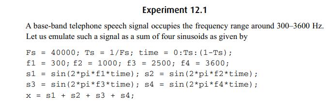
Revisit Experiment 12.1 performing the following tasks:(a) Design a direct-form FIR filter using the following specifications:\[\begin{aligned}A_{\mathrm{p}} & =0.1 \mathrm{~dB} \\A_{\mathrm{r}} & =45 \mathrm{~dB} \\\Omega_{\mathrm{p}} & =2 \pi 9700 \mathrm{~Hz} \\\Omega_{\mathrm{r}}
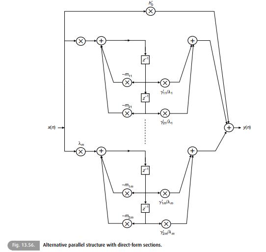
Consider the alternative parallel structure seen in Figure 13.56, whose transfer function is\[H(z)=h_{0}^{\prime}+\sum_{k=1}^{m} \frac{\gamma_{1 k}^{\prime} z+\gamma_{2 k}^{\prime}}{z^{2}+m_{1 k} z+m_{2 k}}\]Discuss the scaling procedure and determine the relative noise variance for this
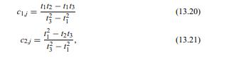
Derive the expressions in Equations (13.20) and (13.21). c2,j= 1112 1113 4-4 (13.20) -1213 4-4 (13.21)
Show that the \(L_{2}\) and \(L_{\infty}\) norms of a second-order \(H(z)\) given by\[H(z)=\frac{\gamma_{1} z+\gamma_{2}}{z^{2}+m_{1} z+m_{2}}\]are as given in Equations (13.28) and (13.29), respectively.
Derive the expressions for the output-noise PSD, as well as their variances, for odd-order cascade filters realized with the following second-order sections:(a) direct-form;(b) optimal state space;(c) state-space free of limit cycles.Assume fixed-point arithmetic.
Repeat Exercise 13.4 assuming floating-point arithmetic.Exercise 13.4Derive the expressions for the output-noise PSD, as well as their variances, for odd-order cascade filters realized with the following second-order sections:(a) direct-form;(b) optimal state space;(c) state-space free of limit
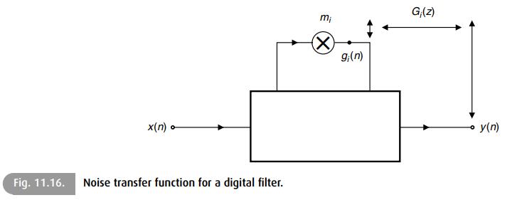
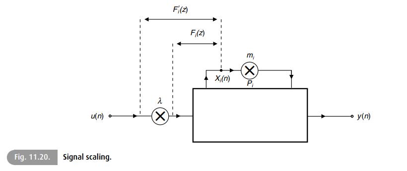
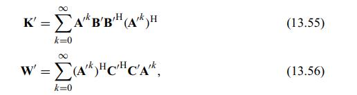
From Equations (13.55), (13.56), and the definitions of \(F_{i}^{\prime}(z)\) and \(G_{i}^{\prime}(z)\) in Figures 11.20 and 11.16 respectively, derive Equations (13.57) and (13.58). x(n) Fig. 11.16. Noise transfer function for a digital filter. mi gi(n) G;(z) y(n)
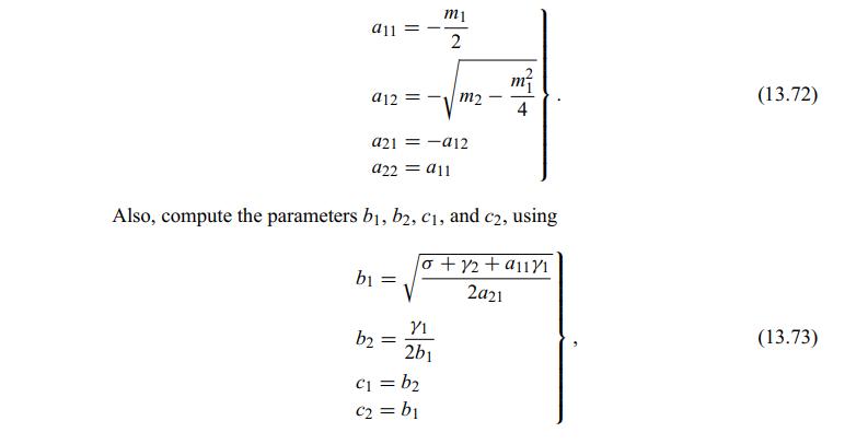
Verify that Equations (13.72)-(13.73) correspond to a state-space structure with minimum output noise. m1 a11=- 2 a12=- m2 - m 4 a21=-a12 a22 = a11 Also, compute the parameters b, b, c1, and c, using bi = o +12+ a111 2a21 V1 b2 = 2b1 c = b2 c = b (13.72) (13.73)
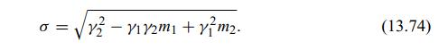
Show that when the poles of a second-order section with transfer function\[H(z)=d+\frac{\gamma_{1} z+\gamma_{2}}{z^{2}+m_{1} z+m_{2}}\]are complex conjugate, then the parameter \(\sigma\) defined in Equation (13.74) is necessarily real. = -V1Y2m+m2. (13.74)
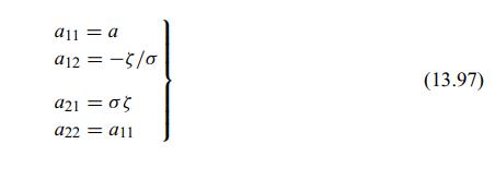
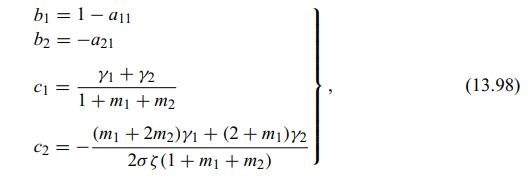
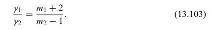
Show that the state-space section free of limit cycles, Structure I, as determined by Equations (13.97) and (13.98), has minimum roundoff noise only if\[\frac{\gamma_{1}}{\gamma_{2}}=\frac{m_{1}+2}{m_{2}-1}\]as indicated by Equation (13.103). a11a a12=-5/0 421 = a22 = a11 (13.97)
Design an elliptic filter satisfying the specifications below:\[\begin{aligned}A_{\mathrm{p}} & =0.4 \mathrm{~dB} \\A_{\mathrm{r}} & =50 \mathrm{~dB} \\\Omega_{\mathrm{r}_{1}} & =1000 \mathrm{rad} / \mathrm{s} \\\Omega_{\mathrm{p}_{1}} & =1150 \mathrm{rad} / \mathrm{s} \\\Omega_{\mathrm{p}_{2}} &
Repeat Exercise 13.10 with the specifications below:\[\begin{aligned}A_{\mathrm{p}} & =1.0 \mathrm{~dB} \\A_{\mathrm{r}} & =70 \mathrm{~dB} \\\omega_{\mathrm{p}} & =0.025 \pi \mathrm{rad} / \mathrm{sample} \\\omega_{\mathrm{r}} & =0.04 \pi \mathrm{rad} / \mathrm{sample} .\end{aligned}\]Exercise
Design an elliptic filter satisfying the specifications of Exercise 13.10, using a cascade of direct-form structures with the ESS technique.Exercise 13.10Design an elliptic filter satisfying the specifications below:\[\begin{aligned}A_{\mathrm{p}} & =0.4 \mathrm{~dB} \\A_{\mathrm{r}} & =50
Design an elliptic filter satisfying the specifications of Exercise 13.10, using parallel connection of second-order direct-form structures, with \(L_{2}\) and \(L_{\infty}\) norms for scaling, employing the closed-form equations of Section 13.2.4.Exercise 13.10Design an elliptic filter satisfying
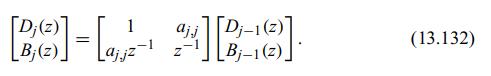
Derive Equation (13.132). Dj(z) Bi(z) [BS]-L-38-3] aj.j Dj- (13.132) Bi-1(z)
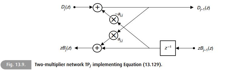
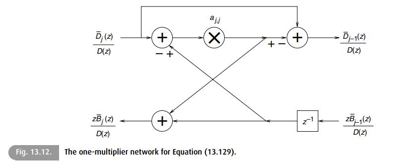
Derive the scaling factor utilized in the two-multiplier lattice of Figure 13.9, in order to generate the one-multiplier lattice of Figure 13.12. + Dj(z) -ajj (X) ajj + zB,(z) Fig. 13.9. Two-multiplier network TP; implementing Equation (13.129). 2-1 Dj-1(2) zBj-1(z)
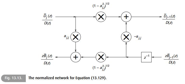
Derive the scaling factor to be used in the normalized lattice of Figure 13.13, in order to generate a three-multiplier lattice. D; (z) D(z) ajj (X) (1-a ( 1/2 zBj (z) D(z) + ( 2,1/2 (1-a) Fig. 13.13. The normalized network for Equation (13.129). + Dj-1(z) D(z) -aj.j IN ZB-1(2) D(z)
Design a two-multiplier lattice structure to implement the filter described in Exercise 13.10.Exercise 13.10Design an elliptic filter satisfying the specifications below:\[\begin{aligned}A_{\mathrm{p}} & =0.4 \mathrm{~dB} \\A_{\mathrm{r}} & =50 \mathrm{~dB} \\\Omega_{\mathrm{r}_{1}} & =1000
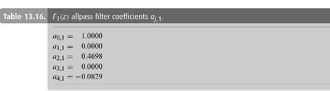
The coefficients of an allpass filter designed to generate doubly complementary filters of order \(N_{1}=5\) are given in Table 13.16. Describe what happens to the properties of these filters when we replace \(z\) by \(z^{2}\). Table 13.16. F1(2) allpass filter coefficients 01. 0,1 1.0000 41.1=
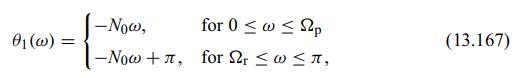
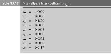
The coefficients of an allpass filter designed to generate doubly complementary filters of order \(N_{1}=9\) are given in Table 13.17.(a) Plot the phase response of the allpass filter and verify the validity of the specifications described in Equation (13.167).(b) Compute the difference in phase
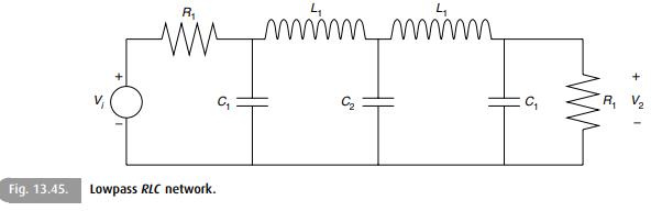
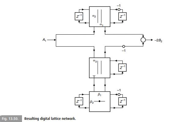
Derive a realization for the circuit of Figure 13.45, using the standard wave digital filter method, and compare it with the wave lattice structure obtained in Figure 13.50, with respect to overall computational complexity. mim_mim C Fig. 13.45. Lowpass RLC network. +1 R
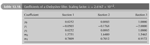
Table 13.18 shows the multiplier coefficients of a scaled Chebyshev filter designed with the following specifications\[\begin{aligned}A_{\mathrm{p}} & =0.6 \mathrm{~dB} \\A_{\mathrm{r}} & =48 \mathrm{~dB} \\\Omega_{\mathrm{r}} & =3300 \mathrm{rad} / \mathrm{s} \\\Omega_{\mathrm{p}}
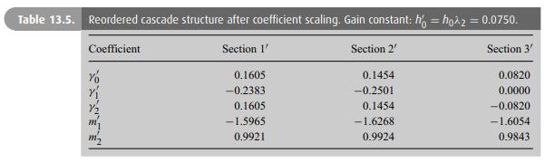
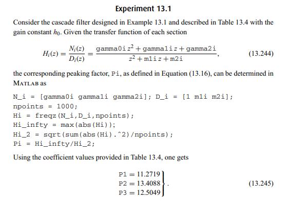
Revisit Experiment 13.1 and determine:(a) The peaking factor and the scaling factors for the 9-bit quantized cascade filter, as described in Table 13.5.(b) The relative output-noise variance for the nonquantized and 9-bit quantized versions of the scaled cascade filter. Table 13.5. Reordered
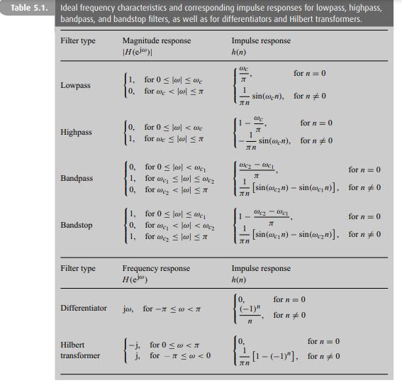
Write a table equivalent to Table 5.1 supposing that the ideal impulse responses have an added phase term of \(-(M / 2) \omega\), for \(M\) odd. Table 5.1. Ideal frequency characteristics and corresponding impulse responses for lowpass, highpass, bandpass, and bandstop filters, as well as for
Assume that a periodic signal has four sinusoidal components at frequencies \(\omega_{0}, 2 \omega_{0}, 4 \omega_{0}, 6 \omega_{0}\). Design a nonrecursive filter, as simple as possible, that eliminates only the components \(2 \omega_{0}, 4 \omega_{0}, 6 \omega_{0}\).
Given a lowpass FIR filter with transfer function \(H(z)\), describe what happens to the filter frequency response when:(a) \(z\) is replaced by \(-z\).(b) \(z\) is replaced by \(z^{-1}\).(c) \(z\) is replaced by \(z^{2}\).
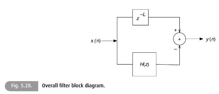
Complementary filters are such that their frequency responses add to a delay. Given an \(M\) th-order linear-phase FIR filter with transfer function \(H(z)\), deduce the conditions on \(L\) and \(M\) such that the overall filter shown in Figure 5.28 is complementary to \(H(z)\). x(n)- Fig. 5.28.
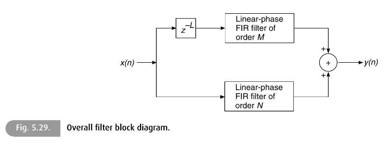
Determine the relationship between \(L, M\), and \(N\) which means that the overall filter in Figure 5.29 has linear phase. Fig. 5.29. x(n) N Linear-phase FIR filter of order M Overall filter block diagram. Linear-phase FIR filter of order N + y(n)
Showing 300 - 400
of 1058
1
2
3
4
5
6
7
8
9
10
11
Step by Step Answers