New Semester
Started
Get
50% OFF
Study Help!
--h --m --s
Claim Now
Question Answers
Textbooks
Find textbooks, questions and answers
Oops, something went wrong!
Change your search query and then try again
S
Books
FREE
Study Help
Expert Questions
Accounting
General Management
Mathematics
Finance
Organizational Behaviour
Law
Physics
Operating System
Management Leadership
Sociology
Programming
Marketing
Database
Computer Network
Economics
Textbooks Solutions
Accounting
Managerial Accounting
Management Leadership
Cost Accounting
Statistics
Business Law
Corporate Finance
Finance
Economics
Auditing
Tutors
Online Tutors
Find a Tutor
Hire a Tutor
Become a Tutor
AI Tutor
AI Study Planner
NEW
Sell Books
Search
Search
Sign In
Register
study help
computer science
digital control system analysis and design
Digital Signal Processing System Analysis And Design 2nd Edition Paulo S. R. Diniz, Eduardo A. B. Da Silva , Sergio L. Netto - Solutions
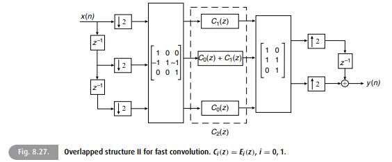
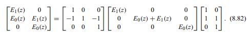
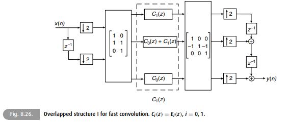
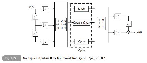
Assume you want to implement an FIR filter of length 16 using the fast convolution structure of Figure 8.27 described by Equation (8.82). Compute the delay and the number of multiplications per sample for decompositions ranging from 3 to 81 subfilters. Fig. 8.27. x(n) 12 C(2) 100 12 -1 1-1 Co(z) +
Implement the transfer function below using the fast convolution structure of Figure 8.27 with the subfilters of length one:\[H(z)=1+z^{-1}+2 z^{-2}+4 z^{-3} .\] x(n) 12 C(z) 100 Co(2) + C(2) 10 121 -1 1-1 00 01 y(n) Fig. 8.27. Co(z) C(2) Overlapped structure Il for fast convolution. C(z) = E(z), i
Implement the transfer function below using the fast convolution structure of Figure 8.27 with the subfilters of length one:\[H(z)=0.25+0.5 z^{-1}-0.5 z^{-2}-0.25 z^{-3} .\] x(n) 12 C(z) 100 Co(2) + C(2) 10 121 -1 1-1 00 01 y(n) Fig. 8.27. Co(z) C(2) Overlapped structure Il for fast convolution.
Design the filter satisfying the following specifications using the minimax approach and show its submatrices of overlapped blocking filtering, for \(M=L=4\) and \(N=2\) :\[\begin{aligned}\delta_{\mathrm{p}} & =0.01 \\\delta_{\mathrm{r}} & =0.005 \\\Omega_{\mathrm{p}} & =0.05 \Omega_{\mathrm{s}}
Design the filter of Exercise 8.26 with the minimax approach and show its submatrices of overlapped blocking filtering for \(M=N=4\) and for \(L=2\).Exercise 8.26Design the filter satisfying the following specifications using the minimax approach and show its submatrices of overlapped blocking
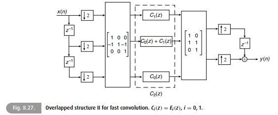
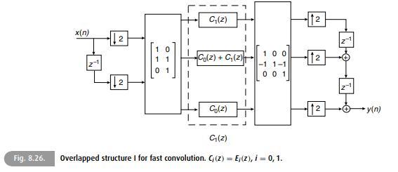
Design the filter of Exercise 8.26 with the WLS approach and derive its overlapped structure I of Figure 8.26.Exercise 8.26Design the filter satisfying the following specifications using the minimax approach and show its submatrices of overlapped blocking filtering, for \(M=L=4\) and \(N=2\)
Design the filter of Exercise 8.26 with the WLS approach and derive its overlapped structure II of Figure 8.27.Exercise 8.26Design the filter satisfying the following specifications using the minimax approach and show its submatrices of overlapped blocking filtering, for \(M=L=4\) and \(N=2\)
Design a filter satisfying the following specifications with the minimax and WLS approaches and show their implementations employing the overlapped structure I of Figure 8.26:\[\begin{aligned}\delta_{\mathrm{p}} & =0.01 \\\delta_{\mathrm{r}} & =0.05 \\\Omega_{\mathrm{p}} & =0.8
Design a filter satisfying the following specifications with the minimax approach and show its submatrices of overlapped blocking filtering for \(M=L=2\) and for \(N=1\) :\[\begin{aligned}\delta_{\mathrm{p}} & =0.01 \\\delta_{\mathrm{r}} & =0.01 \\\Omega_{p_{1}} & =0.48
Solve Exercise 8.31 using the WLS design approach.Exercise 8.31Design a filter satisfying the following specifications with the minimax approach and show its submatrices of overlapped blocking filtering for \(M=L=2\) and for \(N=1\) :\[\begin{aligned}\delta_{\mathrm{p}} & =0.01
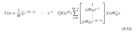
Prove Equation (8.52). Y(z) = -(N-1) 21] C(z) M-I 1 (zWM)- X (zW). 1-0 (WM)-(-1) (8.52)
Show that, for a realization of a WSS process \(\{X\}\) applied as input process to a serial-to-parallel converter, the PSD matrix \(\Gamma_{X}(z)\) is pseudo-circulant.
Let us consider the case where a vector \(\{\mathbf{X}(n)\}\) represents an \(M \times 1\) WSS process, and that\[Y_{i}(n)=W_{i}(n) X_{i}(n)\]for \(i=0,1, \ldots, M-1\). Show that \(\{\mathbf{Y}(n)\}\) is WSS if and only if \(W_{i}(n)=\kappa_{i} \mathrm{e}^{\mathrm{j} \phi_{i} n}\). This result
Show that if you apply an input process WSCS with period \(N\) to a linear periodically time-varying system with period \(N\), the output process will also be WSCS with period \(N\).
Give two distinct realizations for the transfer functions below:(a) \(H(z)=0.0034+0.0106 z^{-2}+0.0025 z^{-4}+0.0149 z^{-6}\).(b) \(H(z)=\left(\frac{z^{2}-1.349 z+1}{z^{2}-1.919 z+0.923}\right)\left(\frac{z^{2}-1.889 z+1}{z^{2}-1.937 z+0.952}\right)\).
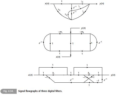
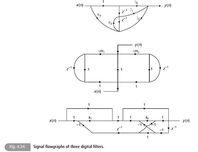
Write the equations that describe the networks in Figure 4.34, by numbering the nodes appropriately. Fig. 4.34. x(n) x(n) 13 % y(n) -m -m x(n) Signal flowgraphs of three digital filters.. y(n) 1 y(n)
Show that:(a) If \(H(z)\) is a Type I filter, then \(H(-z)\) is Type I.(b) If \(H(z)\) is a Type II filter, then \(H(-z)\) is Type IV.(c) If \(H(z)\) is a Type III filter, then \(H(-z)\) is Type III.(d) If \(H(z)\) is a Type IV filter, then \(H(-z)\) is Type II.
Determine the transfer functions of the digital filters in Figure 4.34. Fig. 4.34. x(n) IN 03 32 1 -m 1 x(n) K x(n) -1 % %0 Signal flowgraphs of three digital filters. 1 Z y(n) -m 1 y(n) TN 1 1 y(n) 1
Show that the transfer function of a given digital filter is invariant with respect to a linear transformation of the state vector\[\mathbf{x}(n)=\mathbf{T} \mathbf{x}^{\prime}(n)\]where \(\mathbf{T}\) is any \(N \times N\) nonsingular matrix.
Describe the networks in Figure 4.34 using state variables. Fig. 4.34. x(n) x(n) 13 % y(n) -m -m x(n) Signal flowgraphs of three digital filters.. y(n) 1 y(n)
Implement the transfer function below using a parallel realization with the minimum number of multipliers:\[H(z)=\frac{z^{3}+3 z^{2}+\frac{11}{4}+\frac{5}{4}}{\left(z^{2}+\frac{1}{2} z+\frac{1}{2}\right)\left(z+\frac{1}{2}\right)}\]
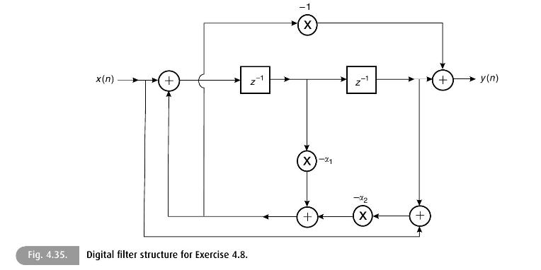
Given the realization depicted in Figure 4.35:(a) Show its state-space description.(b) Determine its transfer function.(c) Derive the expression for its magnitude response and interpret the result. x(n) + Fig. 4.35. Digital filter structure for Exercise 4.8. -1 -x21 Z -1 + y(n) -22 + X +
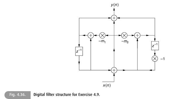
Consider the digital filter of Figure 4.36:(a) Determine its state-space description.(b) Compute its transfer function and plot the magnitude response. y(n) -m -m2 x(n) Fig. 4.36. Digital filter structure for Exercise 4.9.
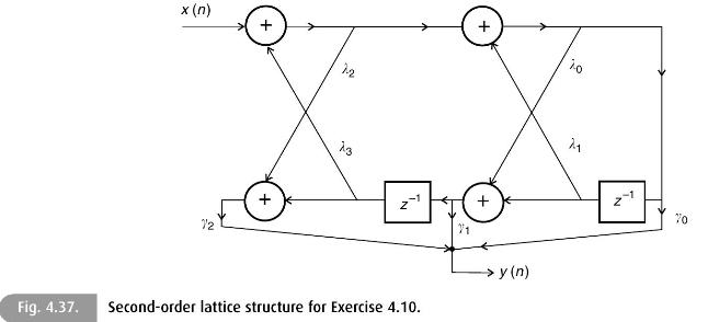
Determine the transfer function of the digital filter shown in Figure 4.37 using the state-space formulation. x (n) 12 + 12 + 13 + y (n) Fig. 4.37. Second-order lattice structure for Exercise 4.10. 1.0 21 70
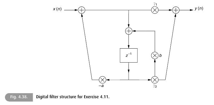
Given the digital filter structure of Figure 4.38:(a) Determine its state-space description.(b) Compute its transfer function.(c) Show its transposed circuit.(d) Use this structure with \(a=-b=\frac{1}{4}\) to design a filter with a unit DC gain to eliminate the frequency \(\omega_{\mathrm{s}} /
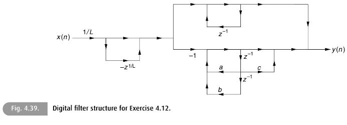
Given the digital filter structure of Figure 4.39:(a) Determine its transfer function.(b) Generate its transposed realization. x(n) Fig. 4.39. 1/L -21/L Digital filter structure for Exercise 4.12. T a b -y(n)
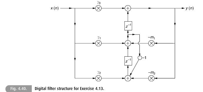
Given the structure shown in Figure 4.40:(a) Determine the corresponding transfer function employing the state-space formulation.(b) Generate its transposed realization.(c) If \(\gamma_{0}=\gamma_{1}=\gamma_{2}\) and \(m_{1}=m_{2}\), analyze the resulting transfer function. x (n) 70 21 -m -m2 72
Find the transpose for each network in Figure 4.34. Fig. 4.34. x(n) x(n) 13 % y(n) -m -m x(n) Signal flowgraphs of three digital filters.. y(n) 1 y(n)
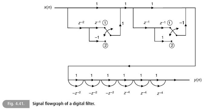
Determine the transfer function of the filter in Figure 4.41, considering the two possible positions for the switches. x(n) -z-2 -z-2 -z-2 z-4 z-4 Fig. 4.41. Signal flowgraph of a digital filter. -Z y(n)
Determine and plot the frequency response of the filter shown in Figure 4.41, considering the two possible positions for the switches. x(n) -z-2 -z-2 -z-2 z-4 z-4 Fig. 4.41. Signal flowgraph of a digital filter. -Z y(n)
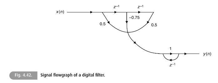
Determine the impulse response of the filter shown in Figure 4.42. x(n) 0.5 z-1 -0.75 0.5 y(n) Z-1 Fig. 4.42. Signal flowgraph of a digital filter.
Show that if two given networks are described by \(Y_{i}=\sum_{j=1}^{M} T_{i j} X_{j}\) and \(Y_{i}^{\prime}=\) \(\sum_{j=1}^{M} T_{i j}^{\prime} X_{j}^{\prime}\), then these networks are interreciprocal if \(T_{j i}=T_{i j}^{\prime}\).
Some FIR filters present a rational transfer function:(a) Show that the transfer function\[H(z)=\frac{\left(r^{-1} z\right)^{-(M+1)}-1}{r e^{\mathrm{j} 2 \pi /(M+1)} z^{-1}-1}\]corresponds to an FIR filter (Lyons, 2007).(b) Determine the operation performed by such a filter.(c) Discuss the general
Plot the pole-zero constellation as well as the magnitude response of the transfer function of Exercise 4.20 for \(M=6,7,8\) and comment on the results.Exercise 4.20Some FIR filters present a rational transfer function:(a) Show that the transfer function\[H(z)=\frac{\left(r^{-1}
Design second-order lowpass and highpass blocks, and combine them in cascade, to form a bandpass filter with passband \(0.3 \leq \omega \leq 0.4\), where \(\omega_{\mathrm{s}}=1\). Plot the resulting magnitude response.
Design second-order lowpass and highpass blocks, and combine them in parallel, to form a bandstop filter with stopband \(0.25 \leq \omega \leq 0.35\), where \(\omega_{\mathrm{s}}=1\). Plot the resulting magnitude response.
Design a second-order notch filter capable of eliminating a \(10 \mathrm{~Hz}\) sinusoidal component when \(\omega_{\mathrm{s}}=200 \mathrm{rad} / \mathrm{sample}\) and show the resulting magnitude response.
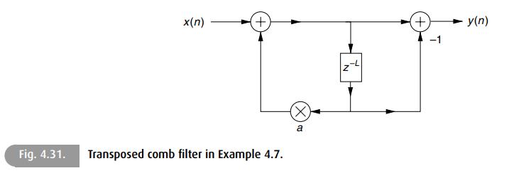
For the comb filter of Figure 4.31, choose \(L=10\) and compute the magnitude and phase responses for the cases where \(a=0, a=0.6\), and \(a=0.8\). Comment on the result. x(n) + Fig. 4.31. Transposed comb filter in Example 4.7. (X) a -L + y(n)
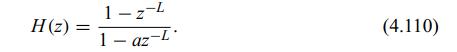
For the comb filter of Equation (4.110), compute the value of the normalization factor that should be multiplied by the transfer function such that the maximum value of the magnitude response becomes 1 . H(z) 1-z-L 1-az-L (4.110)
An FIR filter with the transfer function\[H(z)=\left(z^{-L}-1\right)^{N}\]with \(N\) and \(L\) integers is also a comb filter. Discuss the properties of this filter regarding its zero positions and sharpness.
Given the transfer function\[H(z)=\frac{z\left[z-\cos \left(\omega_{0}\right)\right]}{z^{2}-2 \cos \left(\omega_{0}\right) z+1}\](a) Where are its poles located exactly on the unit circle?(b) Using \(2 \cos \left(\omega_{0}\right)=-2,0,1,2\), and without any external excitation, place an initial
With a state-space structure, prove that, by choosing \(a_{11}=a_{22}=\cos \left(\omega_{0}\right)\) and \(a_{21}=\) \(-a_{12}=-\sin \left(\omega_{0}\right)\), the resulting oscillations in states \(x_{1}(n)\) and \(x_{2}(n)\) correspond to \(\cos \left(\omega_{0} n\right)\) and \(\sin
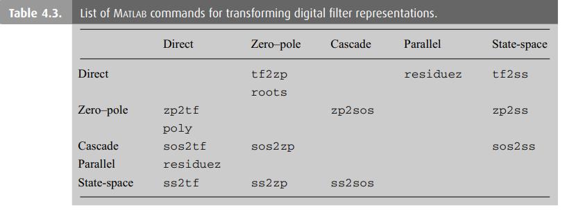
Create Matlab commands to fill in the blanks of Table 4.3. Table 4.3. List of MATLAB commands for transforming digital filter representations. Direct Zero-pole Cascade Direct tf2zp roots Zero-pole zp2tf zp2sos poly Cascade sos2tf sos2zp Parallel residuez State-space ss2tf ss2zp ss2sos Parallel
Characterize the systems below as linear/nonlinear, causal/noncausal and time invariant/time varying:(a) \(y(n)=(n+a)^{2} x(n+4)\)(b) \(y(n)=a x(n+1)\)(c) \(y(n)=x(n+1)+x^{3}(n-1)\)(d) \(y(n)=x(n) \sin (\omega n)\)(e) \(y(n)=x(n)+\sin (\omega n)\)(f) \(y(n)=\frac{x(n)}{x(n+3)}\)(g) \(y(n)=y(n-1)+8
For each of the discrete signals below, determine whether they are periodic or not. Calculate the periods of those that are periodic.(a) \(x(n)=\cos ^{2}\left(\frac{2 \pi}{15} n\right)\)(b) \(x(n)=\cos \left(\frac{4 \pi}{5} n+\frac{\pi}{4}\right)\)(c) \(x(n)=\cos \left(\frac{\pi}{27}
Consider the system whose output \(y(m)\) is described as a function of the input \(x(m)\) by the following difference equations:(a) \(y(m)=\sum_{n=-\infty}^{\infty} x(n) \delta(m-n N)\)(b) \(y(m)=x(m) \sum_{n=-\infty}^{\infty} \delta(m-n N)\).Determine whether the systems are linear and/or time
Compute the convolution sum of the following pairs of sequences:(a) \(x(n)=\left\{\begin{array}{ll}1, & 0 \leq n \leq 4 \\ 0, & \text { otherwise }\end{array} \quad\right.\) and \(\quad h(n)= \begin{cases}a^{n}, & 0 \leq n \leq 7 \\ 0, & \text { otherwise }\end{cases}\)(b)
For the sequence\[x(n)= \begin{cases}1, & 0 \leq n \leq 1 \\ 0, & \text { otherwise }\end{cases}\]compute \(y(n)=x(n) * x(n) * x(n) * x(n)\). Check your results using the MATLAB function conv.
Show that \(x(n)=a^{n}\) is an eigenfunction of a linear time-invariant system by computing the convolution summation of \(x(n)\) and the impulse response of the system \(h(n)\). Determine the corresponding eigenvalue.
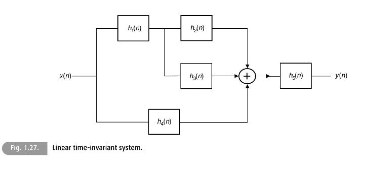
Supposing that all systems in Figure 1.27 are linear and time invariant, compute \(y(n)\) as a function of the input and the impulse responses of each system. x(n) h(n) h(n) h(n) Fig. 1.27. Linear time-invariant system. h(n) + h(n) y(n)
We define the even and odd parts of a sequence \(x(n), \mathcal{E}\{x(n)\}\) and \(\mathcal{O}\{x(n)\}\) respectively, as\[\begin{aligned}\mathcal{E}\{x(n)\} & =\frac{x(n)+x(-n)}{2} \\\mathcal{O}\{x(n)\} & =\frac{x(n)-x(-n)}{2}\end{aligned}\]Show that\[\sum_{n=-\infty}^{\infty}
Find one solution for each of the difference equations below:(a) \(y(n)+2 y(n-1)+y(n-2)=0, y(0)=1\) and \(y(1)=0\)(b) \(y(n)+y(n-1)+2 y(n-2)=0, y(-1)=1\) and \(y(0)=1\).
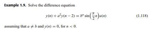
Find the general solution for the difference equation in Example 1.9 when \(a=b\). Example 1.9. Solve the difference equation y(n) + ay(n 2) = b" sin(n)u(n) assuming that ab and y(n) = 0, for n < 0. (1.118)
Determine the solutions of the difference equations below, supposing that the systems they represent are initially relaxed:(a) \(y(n)-\frac{1}{\sqrt{2}} y(n-1)+y(n-2)=2^{-n} \sin \left(\frac{\pi}{4} n\right) u(n)\)(b) \(4 y(n)-2 \sqrt{3} y(n-1)+y(n-2)=\cos \left(\frac{\pi}{6} n\right) u(n)\)(c)
Write a Matlab program to plot the samples of the solutions of the difference equations in Exercise 1.9 from \(n=0\) to \(n=20\).Exercise 1.9Find one solution for each of the difference equations below:(a) \(y(n)+2 y(n-1)+y(n-2)=0, y(0)=1\) and \(y(1)=0\)(b) \(y(n)+y(n-1)+2 y(n-2)=0, y(-1)=1\) and
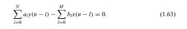
Show that a system described by Equation (1.63) is linear if and only if the auxiliary conditions are zero. Show also that the system is time invariant if the zero auxiliary conditions are defined for consecutive samples prior to the application of any input. N 1=0 M ay(ni) bx(n-1) = 0. - 1=0 (1.63)
Compute the impulse responses of the systems below:(a) \(y(n)=5 x(n)+3 x(n-1)+8 x(n-2)+3 x(n-4)\)(b) \(y(n)+\frac{1}{3} y(n-1)=x(n)+\frac{1}{2} x(n-1)\)(c) \(y(n)-3 y(n-1)=x(n)\)(d) \(y(n)+2 y(n-1)+y(n-2)=x(n)\).
Write a MatLaB program to compute the impulse responses of the systems described by following difference equations:(a) \(y(n)+y(n-1)+y(n-2)=x(n)\)(b) \(4 y(n)+y(n-1)+3 y(n-2)=x(n)+x(n-4)\).
Determine the impulse response of the following recursive system:\[y(n)-y(n-1)=x(n)-x(n-5) .\]
Determine the steady-state response of the system governed by the following difference equation:\[12 y(n)-7 y(n-1)+y(n-2)=\sin \left(\frac{\pi}{3} n\right) u(n) \text {. }\]
Determine the steady-state response for the input \(x(n)=\sin (\omega n) u(n)\) of the filters described by(a) \(y(n)=x(n-2)+x(n-1)+x(n)\)(b) \(y(n)-\frac{1}{2} y(n-1)=x(n)\)(c) \(y(n)=x(n-2)+2 x(n-1)+x(n)\).What are the amplitude and phase of \(y(n)\) as a function of \(\omega\) in each case?
Write a MATLAB program to plot the solution to the three difference equations in Exercise 1.18 for \(\omega=\pi / 3\) and \(\omega=\pi\).Exercise 1.18Determine the steady-state response for the input \(x(n)=\sin (\omega n) u(n)\) of the filters described by(a) \(y(n)=x(n-2)+x(n-1)+x(n)\)(b)
Discuss the stability of the systems described by the impulse responses below:(a) \(h(n)=2^{-n} u(n)\)(b) \(h(n)=1.5^{n} u(n)\)(c) \(h(n)=0.1^{n}\)(d) \(h(n)=2^{-n} u(-n)\)(e) \(h(n)=10^{n} u(n)-10^{n} u(n-10)\)(f) \(h(n)=0.5^{n} u(n)-0.5^{n} u(4-n)\).
Show that \(X_{\mathrm{i}}(\mathrm{j} \Omega)\) in Equation (1.170) is a periodic function of \(\Omega\) with period \(2 \pi / T\).
Suppose we want to process the continuous-time signal\[x_{\mathrm{a}}(t)=3 \cos (2 \pi 1000 t)+7 \sin (2 \pi 1100 t)\]using a discrete-time system. The sampling frequency used is 4000 samples per second. The discrete-time processing carried out on the signal samples \(x(n)\) is described by the
Write a MATLAB program to perform a simulation of the solution of Exercise 1.22.(i) Simulate the continuous-time signals \(x_{\mathrm{a}}(t)\) in MATLAB using sequences obtained by sampling them at 100 times the sampling frequency, that is, as \(f_{\mathrm{s}}(m)=\) \(f_{\mathrm{a}}(m(T / 100))\).
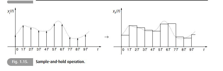
In the conversion of a discrete-time signal to a continuous-time signal, the practical D/A converters, instead of generating impulses at the output, generate a series of pulses \(g(t)\) described by\[\begin{equation*}x_{\mathrm{p}}(t)=\sum_{n=-\infty}^{\infty} x(n) g(t-n T)
Suppose a discrete-time signal \(x(n)\) is obtained by sampling a bandlimited, continuoustime signal \(x_{\mathrm{a}}(t)\) so that there is no aliasing. Prove that the energy of \(x_{\mathrm{a}}(t)\) is equal to the energy of \(x(n)\) multiplied by the sampling period.
Given a sinusoid \(y(t)=A \cos \left(\Omega_{\mathrm{c}} t\right)\), using Equation (1.170), show that if \(y(t)\) is sampled with a sampling frequency slightly above the Nyquist frequency (that is, \(\Omega_{\mathrm{s}}=2 \Omega_{\mathrm{c}}+\epsilon\), where \(\epsilon \ll \Omega_{\mathrm{c}}\)
As seen in Example 1.15, cinema is a three-dimensional spatio-temporal signal that is sampled in time. In modern cinema, the sampling frequency in order to avoid aliasing is \(\Omega_{\mathrm{s}}=24 \mathrm{~Hz}\). However, the persistence of vision is equivalent to a time filter with a bandwidth
Verify that the cross-correlation \(r_{X, Y}\) and the cross-covariance \(c_{X, Y}\) of two random variables \(X\) and \(Y\), as defined in Equations (1.222) and (1.223), satisfy the relation\[c_{X, Y}=r_{X, Y}-E\{X\} E\{Y\} .\] yh(n) =d[c1 sin(n)+c2 cos(n)]. (1.122)
Show that the autocorrelation function of a WSS process \(\{X\}\) presents the following properties:(a) \(R_{X}(0)=E\left\{X^{2}(n)\right\}\)(b) it is an even function; that is: \(R_{X}(v)=R_{X}(-v)\), for all \(v\)(c) it has a maximum at \(v=0\); that is: \(R_{X}(0) \geq\left|R_{X}(v)\right|\),
Show that the autocorrelation function of the output of a discrete linear system with impulse response \(h(n)\) is given by\[R_{Y}(n)=\sum_{k=-\infty}^{\infty} R_{X}(n-k) C_{h}(k)\]where\[C_{h}(k)=\sum_{r=-\infty}^{\infty} h(k+r) h(r)\]
The entropy \(H(X)\) of a discrete random variable \(X\) measures the uncertainty about predicting the value of \(X\) (Cover \(\&\) Thomas, 2006). If \(X\) has the probability distribution \(p_{X}(x)\), its entropy is determined by\[H(X)=-\sum_{x} p_{X}(x) \log _{b} p_{X}(x)\]where the base
For a continuous random variable \(X\) with distribution \(p_{X}(x)\), the uncertainty is measured by the so-called differential entropy \(h(X)\) determined as (Cover \& Thomas, 2006)\[H(X)=-\int_{x} p_{X}(x) \log _{b} p_{X}(x) \mathrm{d} x .\]Determine the differential entropy of the random
Compute the \(z\) transform of the following sequences, indicating their regions of convergence:(a) \(x(n)=\sin (\omega n+\theta) u(n)\)(b) \(x(n)=\cos (\omega n) u(n)\)(c) \(x(n)= \begin{cases}n, & 0 \leq n \leq 4 \\ 0, & n4\end{cases}\)(d) \(x(n)=a^{n} u(-n)\)(e) \(x(n)=\mathrm{e}^{-\alpha n}
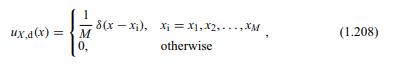
Prove Equation (2.35). z"-1 dz [0, 2j Jc 1, for n #0 for n=0 (2.35)
Suppose that the transfer function of a digital filter is given by\[\frac{(z-1)^{2}}{z^{2}+\left(m_{1}-m_{2}\right) z+\left(1-m_{1}-m_{2}\right)}\]Plot a graph specifying the region of the \(m_{2} \times m_{1}\) plane in which the digital filter is stable.
Compute the impulse response of the system with transfer function\[H(z)=\frac{z^{2}}{4 z^{2}-2 \sqrt{2} z+1}\]supposing that the system is stable.
Compute the time response of the causal system described by the transfer function\[H(z)=\frac{(z-1)^{2}}{z^{2}-0.32 z+0.8}\]when the input signal is the unit step.
Determine the inverse \(z\) transform of the following functions of the complex variable \(z\), supposing that the systems are stable:(a) \(\frac{z}{z-0.8}\)(b) \(\frac{z^{2}}{z^{2}-z+0.5}\)(c) \(\frac{z^{2}+2 z+1}{z^{2}-z+0.5}\)(d) \(\frac{z^{2}}{(z-a)(z-1)}\)(e) \(\frac{1-z^{2}}{\left(2
Compute the inverse \(z\) transform of the functions below. Suppose that the sequences are right handed and one sided.(a) \(X(z)=\sin \left(\frac{1}{z}\right)\)(b) \(X(z)=\sqrt{\frac{z}{1+z}}\).
An alternative condition for the convergence of a series of the complex variable \(z\), namely\[S(z)=\sum_{i=0}^{\infty} f_{i}(z)\]is based on the function of \(z\)\[\begin{equation*}\alpha(z)=\lim _{n \rightarrow \infty}\left|\frac{f_{n+1}(z)}{f_{n}(z)}\right| . \tag{2.261}\end{equation*}\]The
Given a sequence \(x(n)\), form a new sequence consisting of only the even samples of \(x(n)\); that is, \(y(n)=x(2 n)\). Determine the \(z\) transform of \(y(n)\) as a function of the \(z\) transform of \(x(n)\), using the auxiliary sequence \((-1)^{n} x(n)\).
Determine whether the polynomials below can be the denominator of a causal stable filter:(a) \(z^{5}+2 z^{4}+z^{3}+2 z^{2}+z+0.5\)(b) \(z^{6}-z^{5}+z^{4}+2 z^{3}+z^{2}+z+0.25\)(c) \(z^{4}+0.5 z^{3}-2 z^{2}+1.75 z+0.5\).
Given the polynomial \(D(z)=z^{2}-(2+a-b) z+a+1\) that represents the denominator of a discrete-time system:(a) Determine the range of values of \(a\) and \(b\) such that the system is stable, using the stability test described in the text.(b) Plot a graph \(a \times b\), highlighting the stability
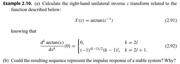
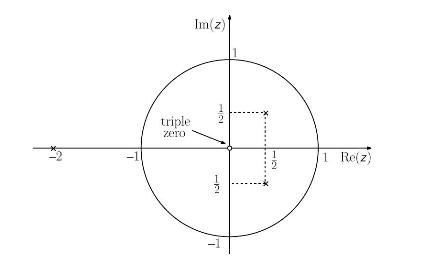
For the pole-zero constellation shown in Figure 2.20, determine the stable impulse response and discuss the properties of the solution obtained.Figure 2.20, -11 Im(z) triple zero 12 11 2 1171 1 Re(z)
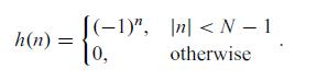
Compute the frequency response of a system with the following impulse response: (-1)", |n]
Compute and plot the magnitude and phase of the frequency response of the systems described by the following difference equations:(a) \(y(n)=x(n)+2 x(n-1)+3 x(n-2)+2 x(n-3)+x(n-4)\)(b) \(y(n)=y(n-1)+x(n)\)(c) \(y(n)=x(n)+3 x(n-1)+2 x(n-2)\).
Plot the magnitude and phase of the frequency response of the digital filters characterized by the following transfer functions:(a) \(H(z)=z^{-4}+2 z^{-3}+2 z^{-1}+1\)(b) \(H(z)=\frac{z^{2}-1}{z^{2}-1.2 z+0.95}\).
If a digital filter has transfer function \(H(z)\), compute the steady-state response of this system for an input of the type \(x(n)=\sin (\omega n) u(n)\).
A given piece of hardware can generate filters with the following generic transfer function:\[H(z)=\frac{\delta_{0}+\delta_{1} z^{-1}-\delta_{2} z^{-1} f(z)}{1-\left(1+m_{1}\right) z^{-1}-m_{2} z^{-1} f(z)}\]where \(f(z)=1 /\left(1-z^{-1}\right)\). Design the filter so that is has unit gain at DC
Given a linear time-invariant system, prove the properties below:(a) A constant group delay is a necessary but not sufficient condition for the delay introduced by the system to a sinusoid to be independent of its frequency.(b) Let \(y_{1}(n)\) and \(y_{2}(n)\) be the outputs of the system to two
Suppose we have a system with transfer function having two zeros at \(z=0\), double poles at \(z=a\), and a single pole at \(z=-b\), where \(a>1\) and \(0
If the signal \(x(n)=4 \cos [(\pi / 4) n-(\pi / 6)] u(n)\) is input to the linear system of Exercise 2.6e, determine its steady-state response.Exercise 2.6e,(e) \(\frac{1-z^{2}}{\left(2 z^{2}-1\right)(z-2)}\).
Compute the Fourier transform of each of the sequences in Exercise 2.1.Exercise 2.1.Compute the \(z\) transform of the following sequences, indicating their regions of convergence:(a) \(x(n)=\sin (\omega n+\theta) u(n)\)(b) \(x(n)=\cos (\omega n) u(n)\)(c) \(x(n)= \begin{cases}n, & 0 \leq n \leq 4
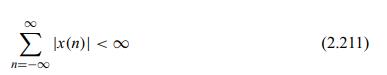
Compute \(h(n)\), the inverse Fourier transform of\[H\left(\mathrm{e}^{\mathrm{j} \omega}\right)=\left\{\begin{aligned}-\mathrm{j}, & \text { for } 0 \leq \omega.\]and show that:(a) Equation (2.211) does not hold.(b) The sequence \(h(n)\) does not have a \(z\) transform. (m) < 00 11=- (2.211)
Prove that the Fourier transform of \(x(n)=\mathrm{e}^{\mathrm{j} \omega_{0} n}\) is given by Equation (2.216) by computing\[X\left(\mathrm{e}^{\mathrm{j} \omega}\right)=\lim _{N \rightarrow \infty} \sum_{n=-N}^{N} x(n) \mathrm{e}^{-\mathrm{j} \omega n}\]
Prove the properties of the Fourier transform of real sequences given by Equations (2.229) to (2.232). Re{X(e)) = Re{X (e-)). (2.229)
State and prove the properties of the Fourier transform of imaginary sequences that correspond to those given by Equations (2.229)-(2.232). Re{X(e)) Re{X (e-j)). (2.229)
Showing 500 - 600
of 1058
1
2
3
4
5
6
7
8
9
10
11
Step by Step Answers