New Semester
Started
Get
50% OFF
Study Help!
--h --m --s
Claim Now
Question Answers
Textbooks
Find textbooks, questions and answers
Oops, something went wrong!
Change your search query and then try again
S
Books
FREE
Study Help
Expert Questions
Accounting
General Management
Mathematics
Finance
Organizational Behaviour
Law
Physics
Operating System
Management Leadership
Sociology
Programming
Marketing
Database
Computer Network
Economics
Textbooks Solutions
Accounting
Managerial Accounting
Management Leadership
Cost Accounting
Statistics
Business Law
Corporate Finance
Finance
Economics
Auditing
Tutors
Online Tutors
Find a Tutor
Hire a Tutor
Become a Tutor
AI Tutor
AI Study Planner
NEW
Sell Books
Search
Search
Sign In
Register
study help
computer science
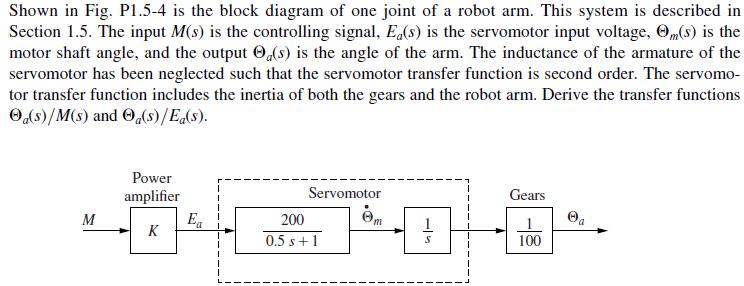
digital control system analysis and design
Digital Control System Analysis And Design 4th Edition Charles Phillips, H. Nagle, Aranya Chakrabortty - Solutions
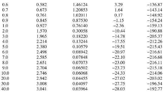
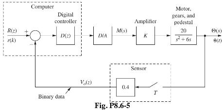
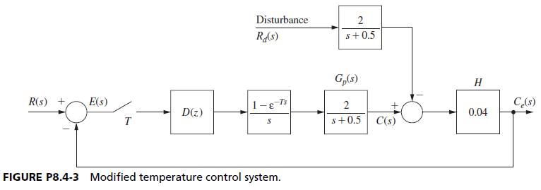
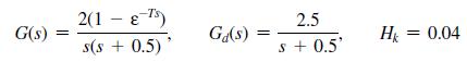
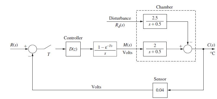
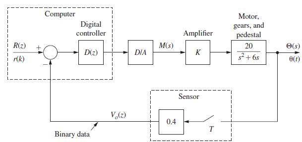
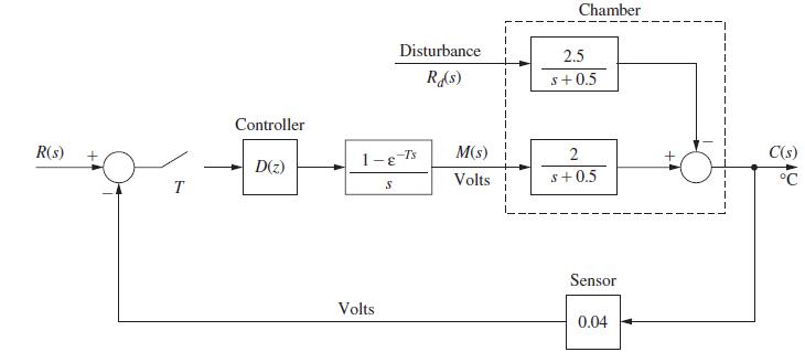
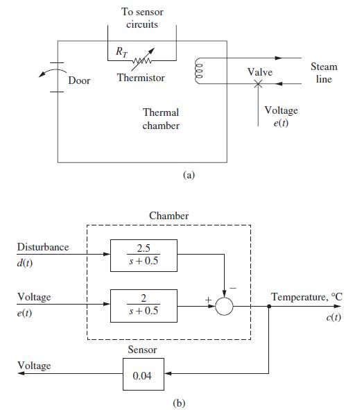
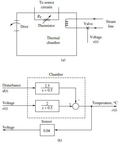
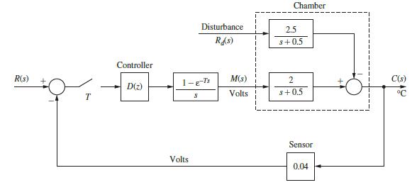
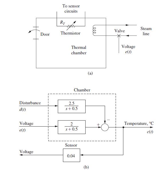
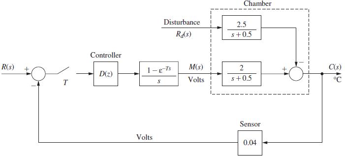
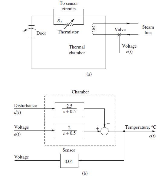
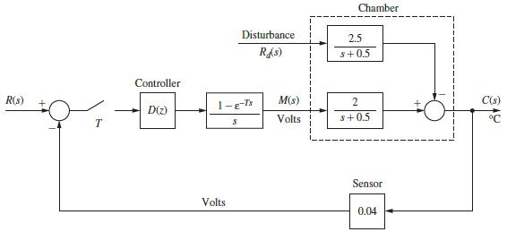
8.4-3. Shown in Fig. P8.4-3 is the block diagram of the temperature control system described in Problem 1.6-1. For this problem, ignore the disturbance input. In Fig. P8.4-3 the sensor gain of \(H=0.04\) has been shifted into the forward path to yield a unity feedback system. The stability
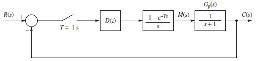
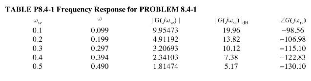
Repeat Problem 8.4-1, using a proportional-plus-integral digital filter.Problem 8.4-1 Consider the system of Fig. P8.2-2 with T = 1 s. The plant frequency response G(jo) is given in Table P8.4-1. (a) Let D(z) = 1. If the system is stable, find its phase margin. (b) Let the digital controller
Repeat Problem 8.6-1, using a proportional-plus-derivative filter.Problem 8.6-1Consider the system of Problem 8.4-1.(a) Design a unity-dc-gain phase-lead compensator that yields a phase margin of approximately 45°.(b) Obtain the system step response of part (a) using MATLAB, and find the rise time
Consider Problem 8.4-2 again. In this problem a proportional-plus-integral (PI) filter is to be designed.(a) The gain added in Problem 8.4-6 to reduce steady-state errors is no longer necessary. Why?(b) Repeat Problem 8.4-6 using a proportional-plus-integral filter, with the gain of 4
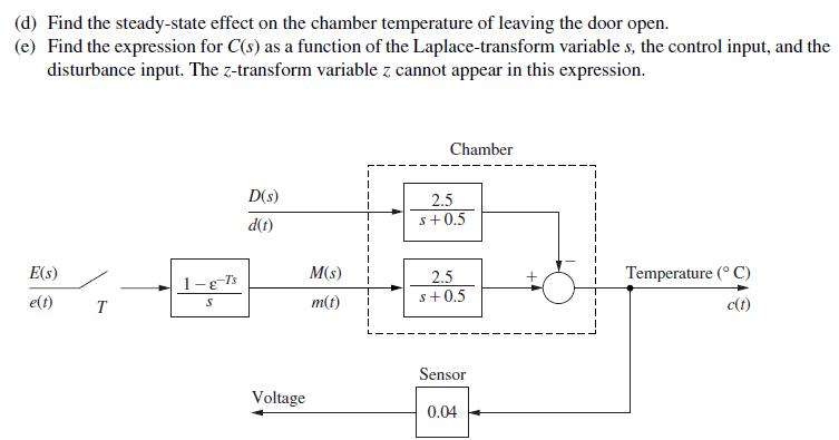
In this problem we consider the effects of the disturbance input in Fig. P8.4-3.(a) Suppose that the disturbance input is a unit step, which models the door to the chamber remaining open. Find the steady-state error in the temperature $c(t)$ for the uncompensated system in Problem 8.4-3.(b) Repeat
(a) Design a PI controller for Problem 8.6-5(b).(b) Design a PD controller for Problem 8.6-5(e).(c) Use the results of parts (a) and (b) to repeat Problem 8.6-5(d).Problem 8.6-5(b) (d) (e)(b) To reduce steady-state errors, K is increased to 5. Design a unity-dc-gain phase-lag controller thatyields
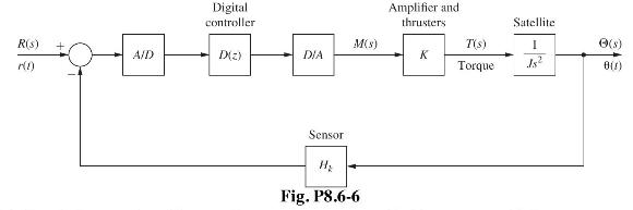
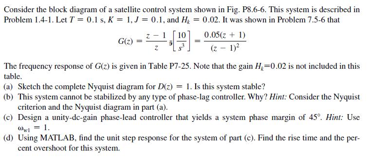
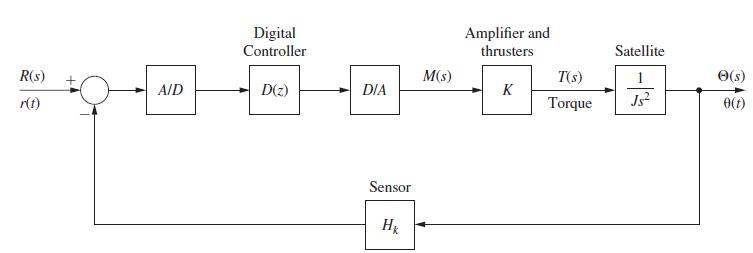
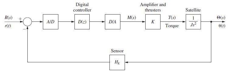
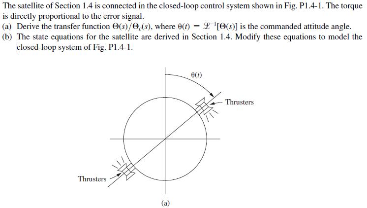
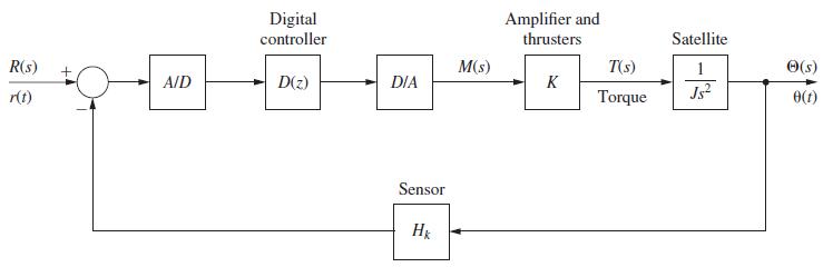
(a) Repeat Problem 8.6-6(a) and (b).(b) Design a PD controller for Problem 8.6-6(c). Use \(\omega_{w 1}=1\).(c) Use the results of part (b) to repeat Problem 8.6-6(d).Problem 8.6-6 Consider the block diagram of a satellite control system shown in Fig. P8.6-6. This system is described in Problem
Consider the chamber temperature control system of Problem 8.4-3. Suppose that a variable gain \(K\) is added to the plant-. The pulse transfer function for this system is given in Problem 8.4-3.(a) Plot the root locus for this system, and find the value of \(K>0\) for which the system is
Consider the system of Problem 8.10-10.(a) Plot the root locus for this system, and find the value of \(K>0\) for which the system is stable.(b) Find the time constant for the system with \(K=1\).(c) Design a phase-lead controller such that the characteristic-equation root in part (b) moves to
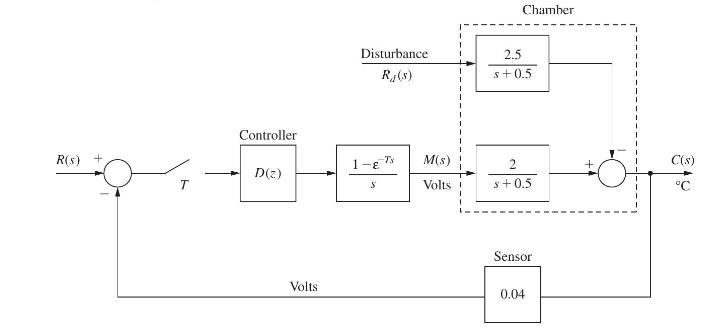
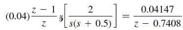
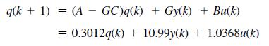
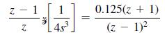
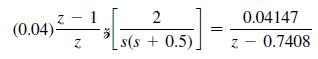
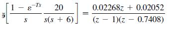
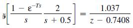
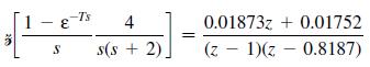
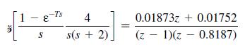
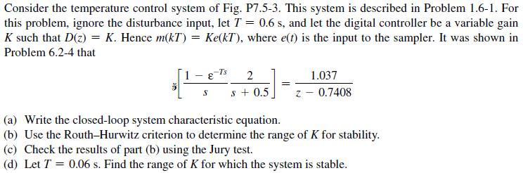
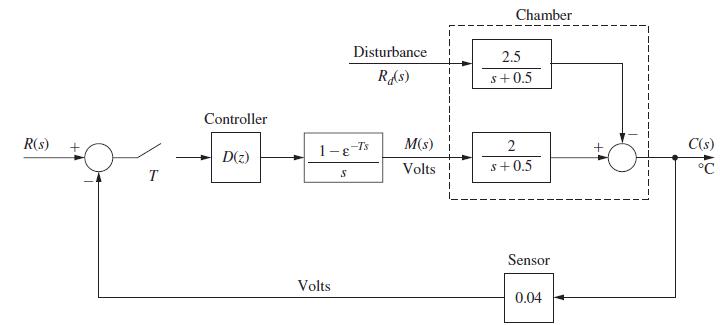
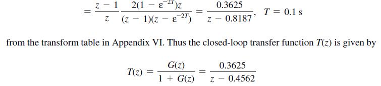
A chamber temperature control system is modeled as shown in Fig. P9.2-3. This system is described in Problem 1.6-1. For this problem, ignore the disturbance input, T=0.6 sT=0.6 s, and let D(z)=1D(z)=1. It was shown in Problem 6.2-4 that((0.04)z−1zz[2s(s+0.5)]=0.04147z−0.7408Note that the
Consider the chamber temperature control system of Problem 9.2-3.(a) Design a predictor observer for this system, with the time constant equal to one-half the value of Problem 9.2-3(b).(b) To check the results of part (a), use (9-46) to show that these results yield the desired observer
Consider the temperature control system of Problem 9.2-3.(a) Determine if this system is controllable.(b) An observer is added to this system in Problem 9.3-2, with the equation [see (9-38)]Construct a single set of state equations for the plant-observer system, with the state vector
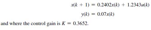
Repeat Problem 9.6-5 for the current observer.Problem 9.6-5Consider the first-order plant described byand a prediction observer described by (9-38). x(k + 1) = Px(k) + Qu(k) y(k) = Rx(k)
For the system of Problem 9.6-5, use a transfer function approach to show that the transfer function Q(z)/U(z)Q(z)/U(z) is first order (even though the system is second order) and is equal to X(z)/U(z)X(z)/U(z). Hence the mode of Q(z)Q(z), which is (A−GC)k(A−GC)k, is not excited by the input
In Problem 9.2-4, a pole-placement design for a satellite control system results in the gain matrix K = [0.194 0.88]. It is desired to have an input signal r(t) applied to the system, so as to realize the system of Fig. 9-12. Write the resulting state equations in the formProblem 9.2-4A satellite
Repeat Problem 9.7-1 for the temperature control system of Problem 9.2-3, where the state equations are given byProblem 9.7-1In Problem 9.2-4, a pole-placement design for a satellite control system results in the gain matrix K = [0.194 0.88]. It is desired to have an input signal r(t) applied to
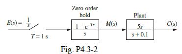
Repeat Problem 4.3-2 for the case that T = 0.1 s and the plant transfer function is given by:Problem 4.3-2(a) Find the system response at the sampling instants to a unit step input for the system of Fig. P4.3-2. Plot c(nT) versus time.(b) Verify your results of (a) by determining the input to
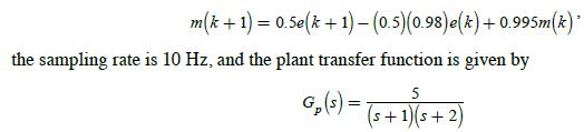
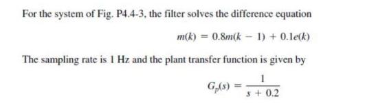
Repeat Problem 4.4-3 for the case that the filter solves the difference equationProblem 4.4-3 m(k+ 1) = 0.5e(k+1) - (0.5)(0.98)e(k) +0.995m(k)* the sampling rate is 10 Hz, and the plant transfer function is given by 5 G (s) = (s+1)(s+2)
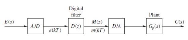
Find the z-transform of the following functions. The results of Problem 4.5-1 may be useful. (a) (c) (e) E(s) = E(s) = E(s) = 20 -0.37s (s+2)(s+5) -1.17s 5+267 s(s+1) (s +55 +6) e-0.37 s(s+4)(s+5) (b) (d) (f) E(s) = Se-0.67s s(s+1) E(s) = -0.2Ts 2 $+267 s (5+1) -0.75Ts 2 E(S) = +25+5
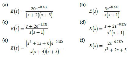
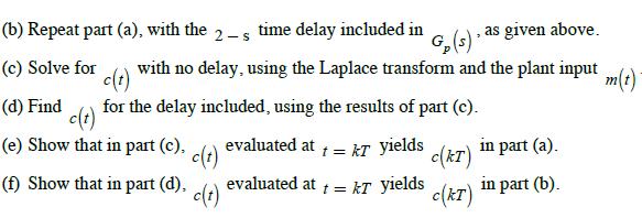
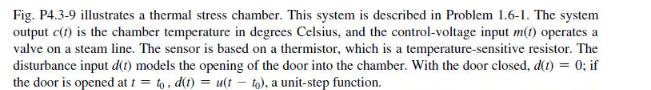
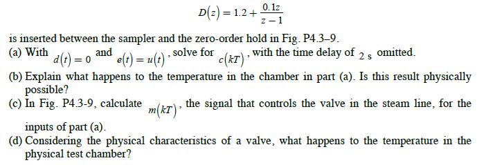
Generally, a temperature control system is modeled more accurately if an ideal time delay is added to the plant. Suppose that in the thermal test chamber of Problem 4.3-9, the plant transfer function is given byProblem 4.3-9 c(s) 2-25 E(S) s+0.5 time delay before its response to an input. For this
For the thermal test chamber of Problems 4.3-9 and 4.6-1, let T = 0.6 s . Suppose that a proportional-integral (PI) digital controller with the transfer functionProblems 4.3-9Problems 4.6-1Generally, a temperature control system is modeled more accurately if an ideal time delay is added to the
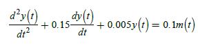
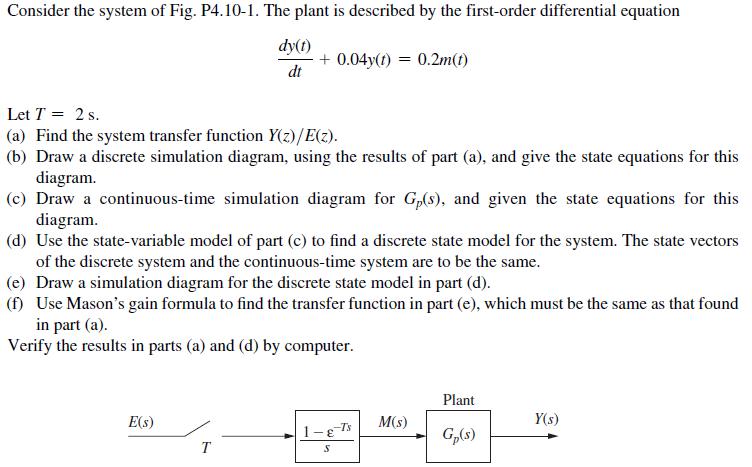
Repeat Problem 4.10-1 for the plant described by the second-order differential equationProblem 4.10-1 dy(t) dt 15 dy(t) + 0.005y(t) = 0.1m(t) dt +0.15-
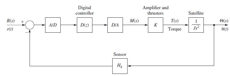
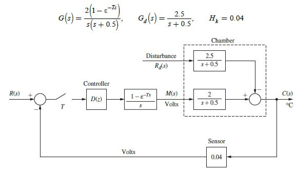
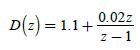
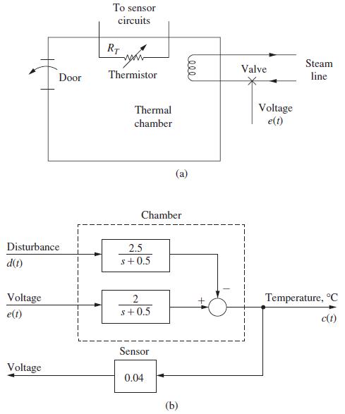
Shown in Fig. P5.3-12 is the block diagram for the temperature control system for a large test chamber. This system is described in Problem 1.6-1. The disturbance shown is the model of the effects of opening the chamber door. The following transfer functions are defined.(a) Derive the transfer
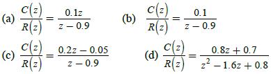
Repeat Problem 5.4-1 for each of the transfer functionsProblem 5.4-1Given a closed-loop system described by the transfer function(a) Express c(k) as a function of r(k), as a single difference equation.(b) Find a set of state equations for this system.(c) Calculate the transfer function from the
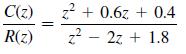
Consider the temperature control system of Problem 5.3-12 and Fig. P5.3-12. Suppose that the digital filter transfer function is given bywhich is a PI (proportional-integral) controller. Suppose that T = 0.6 s , and let Rd(s) = 0 (ignore the disturbance input).(a) Using the closed-loop transfer
Consider the satellite control system of Problem 5.3-14 and Fig. P5.3-14. Let D(z) = 1 , T = 1 s, K = 2 , J = 0.1 , and Hk = 0.02 .(a) Using the closed-loop transfer function, derive a discrete state model for the system.(b) Derive a discrete state model for the plant from the plant transfer
Consider the antenna control system of Problem 5.3-15 and Fig. P5.3-15. Let D(z) = 1, T = 0.05 s , and K = 20 .(a) Using the closed-loop transfer function, derive a discrete state model for the system in the observer canonical form of Fig. 2.6-1.(b) Derive a discrete state model for the plant from
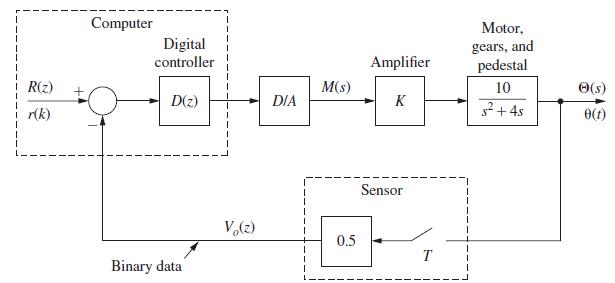
Consider the robot joint control system of Problem 5.3-13 and Fig. P5.3-13. Let D(z) = 1 ,T = 0.1 s, and K = 2.4 .(a) Using the closed-loop transfer function, derive a discrete state model for the system.(b) Derive a discrete state model for the plant from the plant transfer function. Then derive a
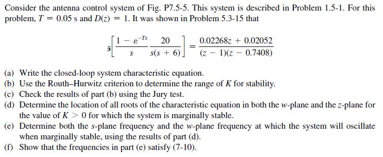
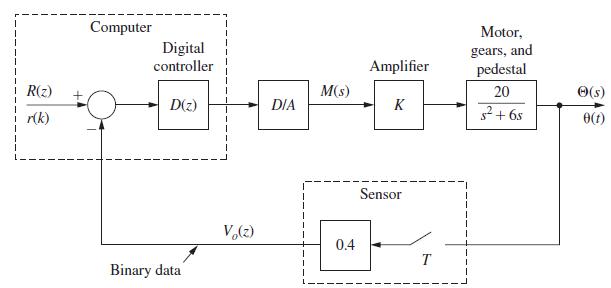
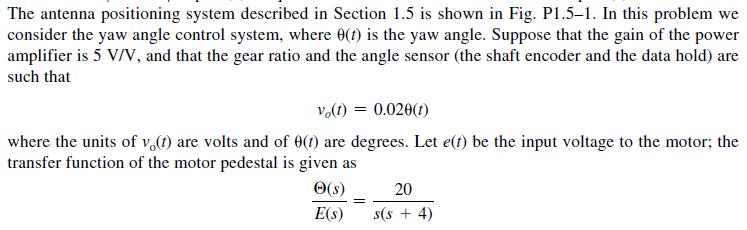
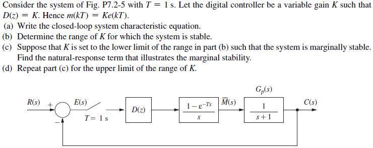
Consider the antenna control system of Fig. P7.5-5. This system is described in Problem 1.5-1. For this problem, T = 0.05 s and D(z) = 1. It was shown in Problem 5.3-15 that(a) Write the closed-loop system characteristic equation.(b) Use the Routh–Hurwitz criterion to determine the range of K
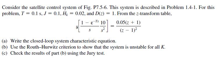
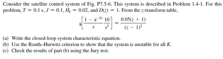
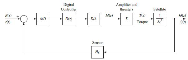
Consider the satellite control system of Fig. P7.5-6. This system is described in Problem 1.4-1. For this problem, T = 0.1 s, J = 0.1, Hk = 0.02, and D(z) = 1. From the z-transform table,(a) Write the closed-loop system characteristic equation.(b) Use the Routh–Hurwitz criterion to show that the
For the system of Problem 7.2-5 and Fig. P7.2-5:(a) Plot the z-plane root locus.(b) Plot the w-plane root locus.(c) Determine the range of K for stability using the results of part (a).(d) Determine the range of K for stability using the results of part (b).Problem 7.2-5Consider the system of
For the chamber temperature control system of Problem 7.5-3 and Fig. P7.5-3:(a) Plot the z-plane root locus.(b) Plot the w-plane root locus.(c) Determine the range of K for stability using the results of part (a).(d) Determine the range of K for stability using the results of part (b).Problem
For the robot arm joint control system of Problem 7.5-4 and Fig. P7.5-4:(a) Plot the z-plane root locus.(b) Plot the w-plane root locus.(c) Determine the range of K for stability using the results of part (a).(d) Determine the range of K for stability using the results of part (b).Problem
For the satellite control system of Problem 7.5-6 and Fig. P7.5-6:(a) Plot the z-plane root locus.(b) Plot the w-plane root locus.(c) Determine the range of K for stability using the results of part (a).(d) Determine the range of K for stability using the results of part (b).Problem 7.5-6
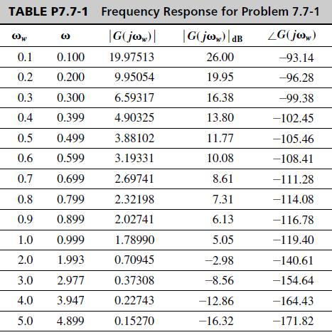
For the robot arm joint control system of Problem 7.5-4 and Fig. P7.5-4, let K = 1 .(a) The frequency response for G(z) was calculated by computer and is given in Table P7.7-1.Sketch the Nyquist diagram for the open-loop function G(z)Hk , with Hk = 0.07 ⇒ − 23.1 dB .(b) Determine the
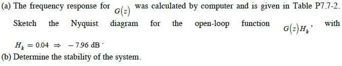
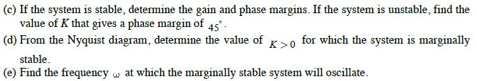
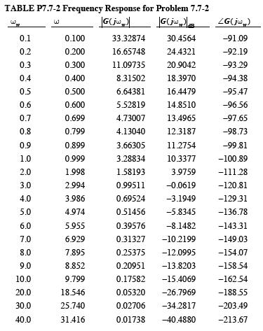
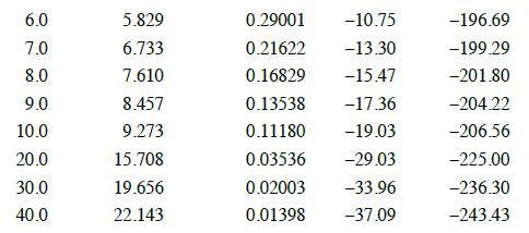
For the antenna control system of Problem 7.5-5 and Fig. P7.5-5, let K = 1 .Problem 7.5-5 (a) The frequency response for was calculated by computer and is given in Table P7.7-2. G(z) Sketch the Nyquist diagram for the open-loop function with G(z) H' H = 0.04 -7.96 dB (b) Determine the stability of
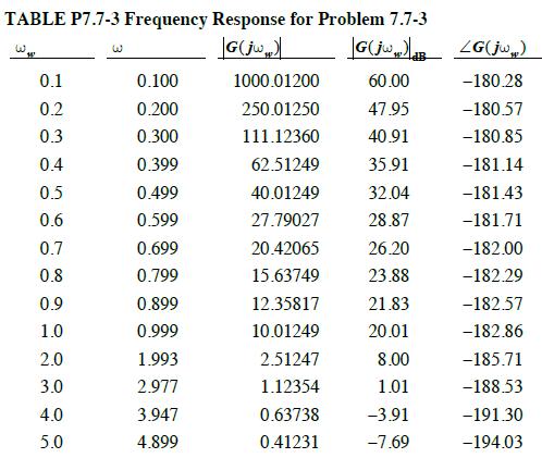
For the satellite control system of Problem 7.5-6, the frequency response for G(z) was calculated by computer and is given in Table P7.7-3.(a) Sketch the Nyquist diagram for the open-loop function G(z)H , with H = 0.02 ⇒ − 34.0 dB .(b) Use the results in part (a) to determine the range of K
For the antenna control system of Problem 7.5-5 and Fig. P7.5-5:(a) Plot the z-plane root locus.(b) Plot the w-plane root locus.(c) Determine the range of K for stability using the results of part (a).(d) Determine the range of K for stability using the results of part (b).Problem 7.5-5Problem
For the system of Problem 7.2-5 and Fig. P7.2-5, let K = 1 .(a) Determine the stability of the system.(b) Sketch the Bode diagram, and use this diagram to sketch the Nyquist diagram.(c) If the system is stable, determine the gain and phase margins. If the system is unstable, find the value of K
For the temperature control system of Problem 7.5-3 and Fig. P7.5-3, let K = 1 .(a) Determine the stability of the system.(b) Plot the Bode diagram, and the Nyquist diagram.(c) If the system is stable, determine the gain and phase margins. If the system is unstable, find the value of K that
The thermal chamber transfer function C(s) E(s) = 2 (s + 0.5) of Problem 1.6-1 is based on the units of time being minutes.(a) Modify this transfer function to yield the chamber temperature c(t) based on seconds.(b) Verify the result in part (a) by solving for c(t) with the door closed and the
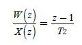
(a) The transfer function for the right-side rectangular-rule integrator was found in Problem 2.2-1 to be Y(z)/X(z) = Tz/(z −1) . We would suspect that the reciprocal of this transfer function should yield an approximation to a differentiator. That is, if w(kT) is a numerical derivative of x(t)
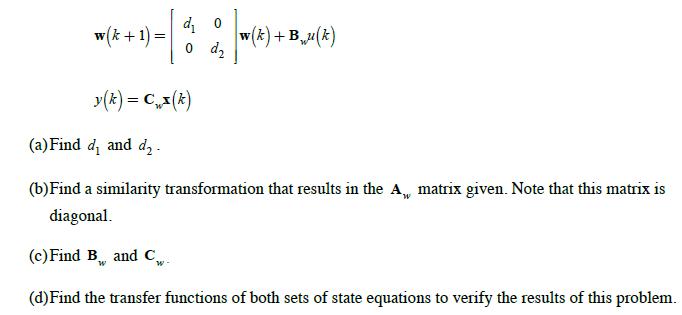
Consider the system of Problem 2.10-2. A similarity transformation on these equations yields d w(k+ 1) = y (k) = C(k) 22 w(k)+ Bu(k) d (a) Find d, and d. (b) Find a similarity transformation that results in the A,, matrix given. Note that this matrix is diagonal. (c) Find B and C (d) Find the
Repeat Problem 2.10-2 for the system described by(a) Find the transfer function Y(z)/U(z).(b) Using any similarity transformation, find a different state model for this system.(c) Find the transfer function of the system from the transformed state equations.(d) Verify that A given and Aw
Consider the system described in Problem 2.10-2.(a) Find the transfer function of this system.(b) Let u(k) = 1, k ≥0 (a unit step function) and x(0) = 0 . Use the transfer function of part (a) to find the system response.(c) Find the state transition matrix Φ(k) for this system.(d) Use
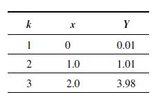
Suppose that a square-law circuit has the input–output relationshipwhere x is the input voltage and y is the output voltage.(a) Derive a least-squares procedure for calculating k.(b) Experimentation with the circuit yields the following data pairs:Find the least-squares value for k for these
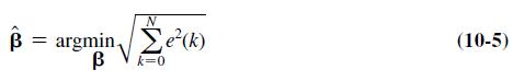
Equation (10-5) gives a least-squares estimate for curve fitting. This equation was derived by finding the point at which the slope of the cost function is zero. The maximum of a function also occurs at the point at which the slope is zero. Show that (10-5) is a minimum, not a maximum, of the cost
Consider the sinusoidal function y(k) = sin (10 k) for k = 0, 1, . . . , 9. Find the minimum degree of the polynomial which fits this function with a maximum least-squares error of 10-3.
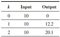
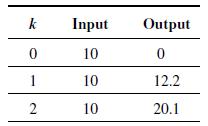
Using the data given in Problem 10.5-1, derive the state-variable model using the algorithm described in Section 10.4.Problem 10.5-1(a) A first-order system yields the following input–output measurements:Find the system transfer function by the least-squares batch procedure, using all the
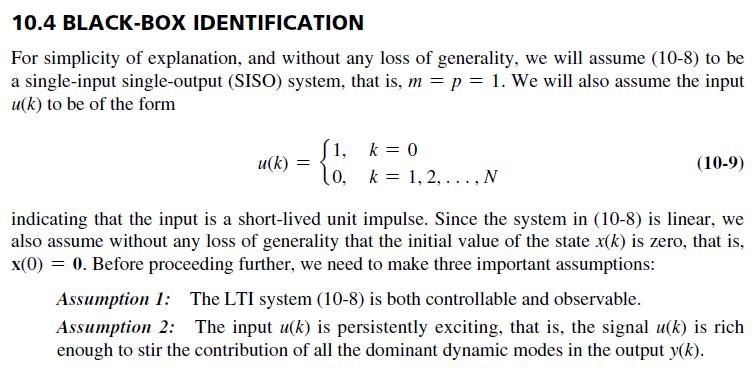
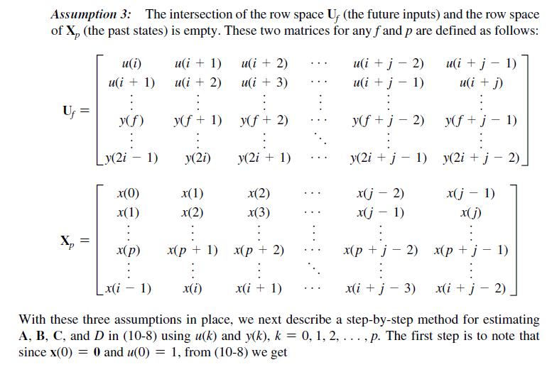
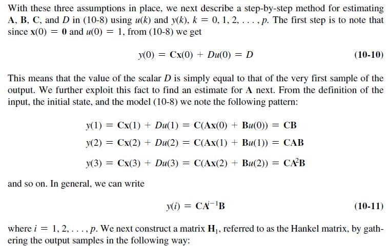
Derive the SISO black-box identification algorithm described in Section 10.4 when the excitation input u(k) is a unit step signal.SISO black-box 10.4 BLACK-BOX IDENTIFICATION For simplicity of explanation, and without any loss of generality, we will assume (10-8) to be a single-input single-output
Consider the SISO continuous-time model:Assume u(k) to be an impulse input. Sample this system with T = 10 s, 1 s, and 0.1 s, and compare how accurately the estimated impulse responses, computed using the black-box identification method of Section 10.4, for each case match the measured response
(a) A first-order system yields the following input–output measurements:Find the system transfer function by the least-squares batch procedure, using all the data.(b) An additional data pair for k = 3 is measured, with the input equal to zero and the output equal to 31.8. Start the recursive
For a third-order discrete system, suppose that the data pairs [u(k), y(k)], k = 0, 1,g5, are available.In these data, u(k) is the input and y(k) is the output. Write the complete expression for FT(N)y(N) as in (10-43), using all the data.Equation 10-43 ALS [FT(N)F(N)] FT (N)y(N) = (10-43)
Derive (10-47), the weighted least-squares estimate.Equation 10-47 WLS = [FT(N)W(N)F(N)]F(N)W(N)y(N) (10-47)
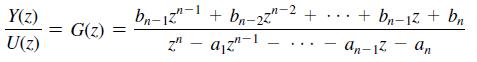
Consider that b1, b2,g, bm in (10-30) for some given positive integer m are all known constants. Using the method proposed in Section 10.6 re-derive (10.43) to compute the least-squares estimate of only the unknown coefficients of (10-30).Equation 10-30Equation 10.43 Y(z) U(z.) = G(z) bn-12"-1 +
Using (10-47), (10-52), (10-56), and (10-57), derive the equations for the recursive least-squares estimation, (10-59)–(10-61). OWLS = [FT(N)W(N)F(N)JFT(N)W(N)y(N) (10-47)
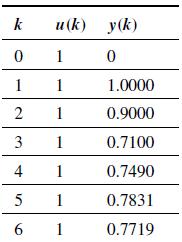
Using the MATLAB function awgn, repeat the recursive least-squares estimation of Example 10.4 when the output is corrupted by a white Gaussian noise with 10.0 dB SNR. Compare the estimation results with those for 1.0 dB SNR.Example 10.4Consider the input and output data of a LTI system with
Consider the values of y(k) in Problem 10.6-3 at k = 0, 2, 4, 6, and 8. Using these values and assuming T = 0.2 s, repeat the least-squares estimation of the transfer function. Next, consider the values at k = 0, 4, and 8, and assuming T = 0.4 s repeat the estimation one more time. Compare both of
Consider the transfer functionExcite this transfer function with the following inputs, and collect the respective outputs in a vector y(k), k = 0, 1, . . . , 20. Assume the sampling time T = 0.1 s.(a) u(k) = sin (10k)(b) u(k) = 100 sin (10k)(c) u(k) = sin (10k) + sin (20k)(d) u(k) = sin (k) +
Given that (11-21) and (11-22) are valid, derive (11-23). S S + x(N-1)Q(N-1)x(N-1) + u(N-1)R(N 1)u(N 1) = (11-21)
Show that (11-35) can also be expressed as P(Nm) = A[P(Nm +1) P(N m + 1)BDB/P(N m + 1)]A + Q - where D= [B'P(Nm + 1)B + RJ-. -
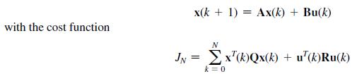
Given the discrete systemshow that the optimal gains which minimize JN are unchanged if the elements both in Q and in R are multiplied by the positive scalar β. with the cost function x(k+1) = Ax(k) + Bu(k) JN = = x(k)Qx(k) + u(k)Ru(k) k = 0
Given the first-order plant described by(a) Calculate the feedback gains required to minimize the cost function, using the partial-differentiation procedure of Section 11.3.(b) Repeat part (a) using the difference-equation approach of Section 11.4.(c) Find the maximum magnitude of u(k) as a
Consider the third-order continuous-time LTI system with A = 208 0 0 0 3 0 -8 -6 x = Ax + Bu y = Cx 0 B = 0, and C= [1 0 0]. Using = 8 0 0 0 6 0 0 4 3 R = 1.5 (a) First design a LQ controller for this continuous time-system using the MATLAB function lqr. Let the optimal controller gain vector be K.
Given a general first-order plant described by(a) Show that for R = 0, the optimal gain K(k) is constant for all k ≥ 0.(b) Give the input sequence u(k), k ≥ 0, for part (a), where u(k) is a function of x(0).(c) Draw a flow graph of the closed-loop system for part (a).(d) Give the
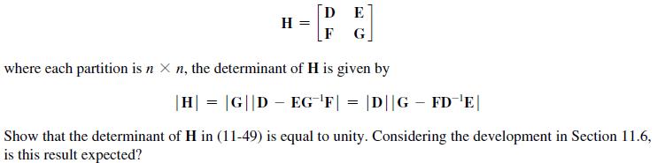
It is shown in [6] that given the partitioned matrix H = D E F G where each partition is n X n, the determinant of H is given by |H| = |G||D EGF| = |D||G FDE| Show that the determinant of H in (11-49) is equal to unity. Considering the development in Section 11.6, is this result expected?
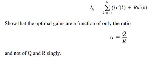
Give a first-order time-invariant discrete system with a cost function N JN = Qx(k) + Ru(k) k = 0 Show that the optimal gains are a function of only the ratio Q R and not of Q and R singly. =
The system considered here is the classical system of Doyle and Stein [9] to illustrate robustness problems. The system of Doyle and Stein is analog; the discrete model of the system is used here [11]. The sample period, T = 0.006 s, was chosen small so that the results approximate those of Doyle
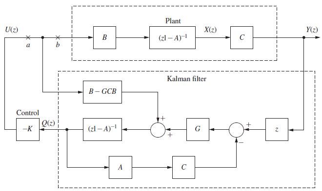
For the IH-LQG control system of Fig. 11-6, suppose that the plant is single-input single-output, such that B and C are vectors. To determine the system robustness, the open-loop transfer functions for the system opened at a and opened at b must be determined.(a) Find the open-loop transfer
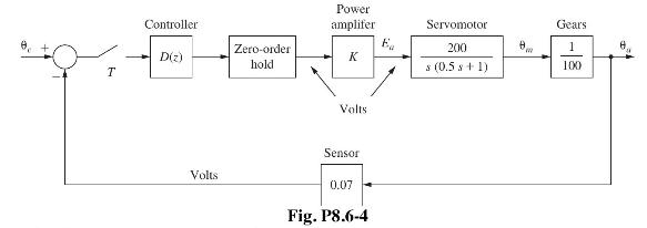
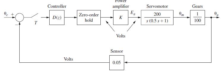
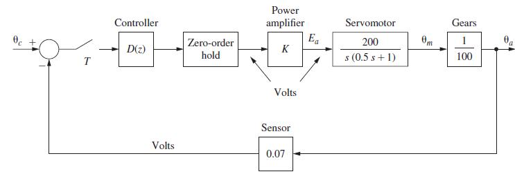
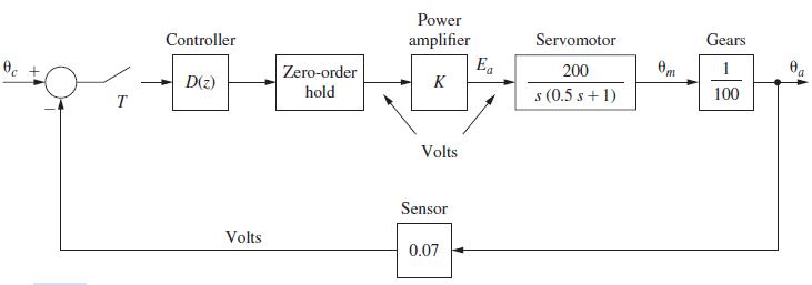
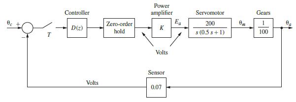
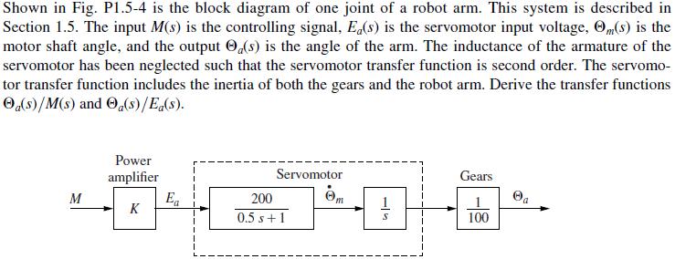
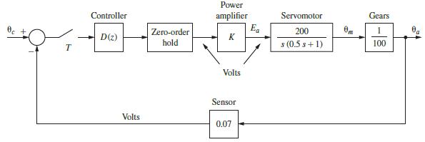
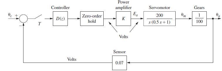
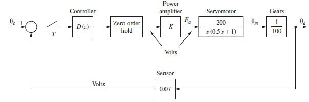
Consider the robot-joint control system of Fig. P5.3-13. This system is described in Problem 1.5-4.Problem 1.5-4 T Controller D(z) Volts Power Zero-order hold Servomotor Ea 200 100 s (0.5 s + 1) amplifier K Volts Sensor 0.07 0m Gears 100
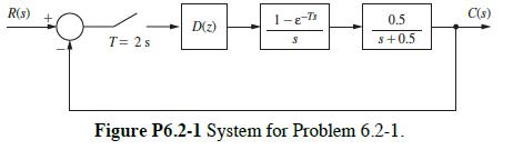
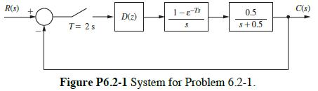
Consider the closed-loop system of Fig. P6.2-1.(a) Calculate and plot the unit-step response at the sampling instants, for the case that D(z) = 1 .(b) Calculate the system unit-step response of the analog system, that is, with the sampler, digital controller, and data hold removed. Plot the
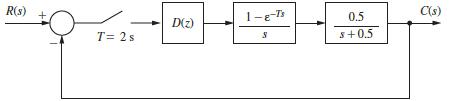
Consider the system of Fig. P6.2-1, with D(z) = 1 . Use the results of Problem 6.2-1 if available.(a) Find the system time constant τ for T = 2 s .(b) With the input a step function, find the time required for the system output c(kT) to reach 98 percent of its final value, for T = 2 s . Recall
In Example 6.1 the response of a sampled-data system between sample instants was expressed as a sum of delayed step responses.(a) Use this procedure to find the system output y(t) of Fig. P6.2-1 at t = 1 s .(b) Repeat part (a) at t = 3 s .(c) The equation for c(t) in part (a) and that for c(t)
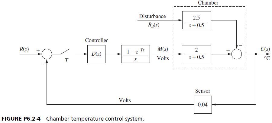
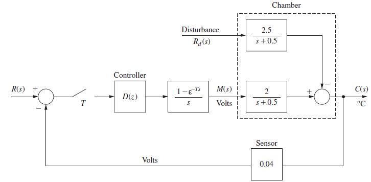
Shown in Fig. P6.2-4 is the block diagram of a temperature control system for a large test chamber. This system is described in Problem 1.6-1. Ignore the disturbance input for this problem.(a) With D(z) = 1 and T = 0.6 s , evaluate and plot the system response if the input is to command a 10°C
Consider the temperature control system of Problem 6.2-4 and Fig. P6.2-4.(a) Let T = 6 s , and solve for the response to the input R(s) = 0.4 s−1 . Plot this response on the same graph with the response found in Problem 6.2-4. Note the effects of increasing T from 0.6 s to 6 s, when the plant
Consider the system of Fig. P6.2-4, with D(z) = 1 . Use the results of Problems 6.2-4 and 6.2-5 if available.(a) Find the system time constant τ for T = 0.6 s .(b) With the input a step function, find the time required for the system output c(kT) to reach 98 percent of its final value. Note that
The block diagram of a control system of a joint in a robot arm is shown in Fig. P6.2-7. This system is discussed in Section 1.6. Let T = 0.1 s and D(z) = 1 .(a) Evaluate C(z) if the input is to command a 20°C step in the output and K = 10. Note that the system input must be a step function with
The block diagram of a control system of a joint in a robot arm is shown in Fig. P6.2-7. Let T = 0.1 s , K = 10 , and D(z) = 1 . The results of Problem 6.2-7 are useful in this problem if these results are available.(a) Find the damping ratio ζ , the natural frequency ωn , and the time constant
The block diagram of an attitude control system of a satellite is shown in Fig. P6.4-2. Let T = 1 s , K = 100 , J = 0.1 , Hk = 0.02 , and D(z) = 1.(a) Find the damping ratio ζ the natural frequency ωn , and the time constant τ of the open-loop system. If the system characteristic equation has
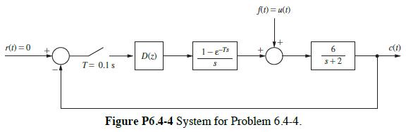
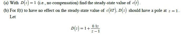
Consider the system of Fig. P6.4-4. This system is called a regulator control system, in which it is desired to maintain the output, c(t) , at a value of zero in the presence of a disturbance, f (t) . In this problem the disturbance is a unit step. r(t)=0 T= 0.1 s D(z) 1-e-Ts S f(t) = u(t) Figure
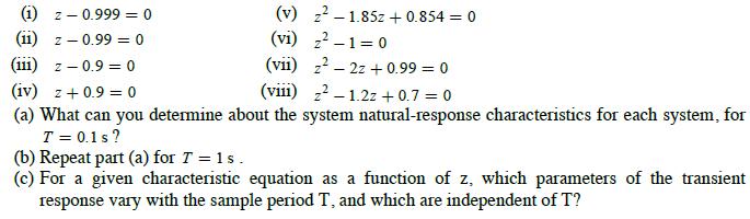
Consider the sampled-data systems with the following characteristic equations: (1) 2- - 0.999 = 0 Z-0.99 = 0 (v) 21.85z + 0.854 = 0 (vi) 2-1=0 (vii) 22z+0.99 = 0 (11) (111) z - 0.9=0 (iv) z +0.9 = 0 (viii) z-1.22 +0.7 = 0 (a) What can you determine about the system natural-response characteristics
Consider the system of Fig. P6.2-1. Suppose that an ideal time delay of 0.2 s is added to the plant, such that the plant transfer function is now given by(a) Find the time constant τ of the system if the time delay is omitted.(b) Find the time constant τ of the system if the time delay is
(a) Give the system type for the following systems, with D(z) = 1. It is not necessary to find the pulse transfer functions to find the system type. Why?(i) Fig. P6.2-1.(ii) Fig. P6.2-4.(iii) Fig. P6.2-7.(iv) Fig. P6.4-2.(v) Fig. P6.4-4.(b) It is desired that the systems of part (a) have zero
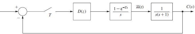
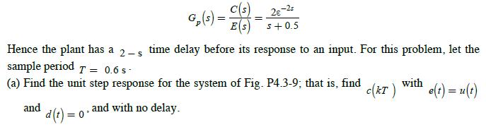
Consider the system of Fig. P6.5-2. The digital filter is described by(a) Find the system type.(b) Find the steady-state response for a unit-step input, without finding C(z).(c) Find the approximate time for the system to reach steady state.(d) Find the unit-step response for the system and
Consider the system of Fig. P6.5-2, with D(z) = 1 .(a) With the sampler and zero-order hold removed, write the system differential equation.(b) Using the rectangular rule for numerical integration with the numerical integration increment equal to 0.25 s, evaluate the unit-step response for 0 ≤
Consider the numerical integration of the differential equation (6-24) in Section 6.6. Applying the rectangular rule results in the difference equation (6-25), which can be expressed as(a) Use the z-transform to solve this equation as a function of x(0) and H.(b) Use the results of part (a) to
Consider the numerical integration of the differential equationusing the rectangular rule.(a) Develop the difference equation, as in (6-25), for the numerical integration of this differential equation.(b) Let r(t) = 1 , x(0) = 0 , and H = 0.1 . Use the z-transform to solve the difference equation
Consider the numerical integration of the differential equationusing the predictor-corrector of Section 6.6. The predictor method is the rectangular rule, and the corrector method is the trapezoidal rule.(a) Develop the difference equation, using (6-32) through (6-35), for the numerical
Consider the numerical integration of the differential equationusing the predictor-corrector of Section 6.6. The predictor method is the rectangular rule, and the corrector method is the trapezoidal rule.(a) Develop the difference equation, for the numerical integration of the given differential
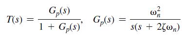
Consider the second-order analog system described byExtra \left or missing \rightwhere T(s)T(s) is the closed-loop transfer function and Gp(s)Gp(s) is the plant transfer function. Show that the phase margin ϕmϕm and the damping ratio ζζ are related by ϕm≈100ζϕm≈100ζ by sketching this
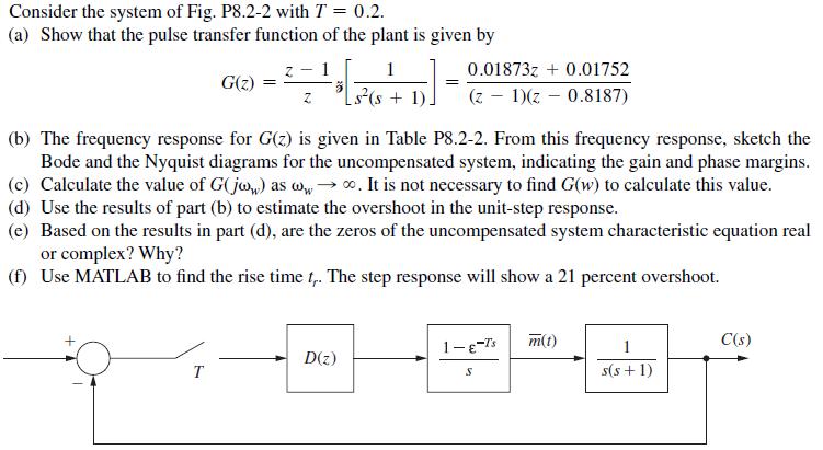
Consider the system of Fig. P8.2-2 with T=0.2T=0.2.(a) Show that the pulse transfer function of the plant is given byExtra \left or missing \right(b) The frequency response for G(z)G(z) is given in Table P8.2-2. From this frequency response, sketch the Bode and the Nyquist diagrams for the
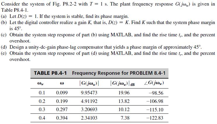
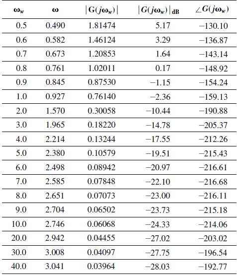
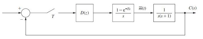
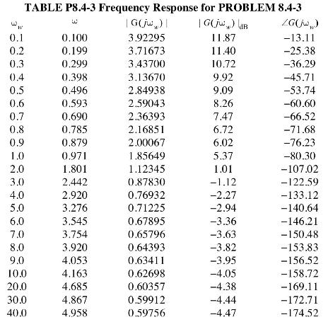
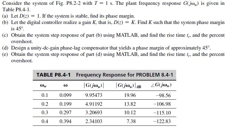
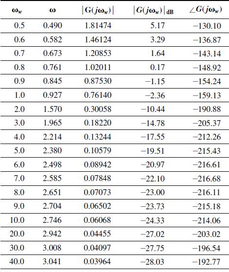
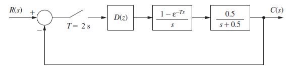
Consider the system of Fig. P8.2-2 with T=1T=1 s. The plant frequency response Extra close brace or missing open brace is given in Table P8.4-1.(a) Let D(z)=1D(z)=1. If the system is stable, find its phase margin.(b) Let the digital controller realize a gain KK, that is, D(z)=KD(z)=K. Find KK such
This problem is based on the solution in Problem 8.4-3. Suppose that in Fig. P8.4-3, the sensor gain \(H=0.04\) is moved back to the feedback path. What effect does this have on the percent steady-state error of Problem 8.4-3, where this error is defined as\[\text { steady-state error }=\frac{\text
Consider the system of Problem 8.4-1.(a) Design a unity-dc-gain phase-lead compensator that yields a phase margin of approximately \(45^{\circ}\).(b) Obtain the system step response of part (a) using MATLAB, and find the rise time \({ }_{t_{r}}\) and the percent overshoot.(c) Compare the
Repeat Problem 8.4-2 using a phase-lead controller. In part (c), the overshoot is approximately 26 percent.Problem 8.2-2 Consider the system of Fig. P8.2-2 with T = 0.2. (a) Show that the pulse transfer function of the plant is given by 1 Z s(s+ 1). G(z) T = z 1 = (b) The frequency response for
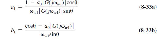
Three constraints are given on the choice of the phase-margin frequency, \(\omega_{w 1}\), in Section 8.6 for phase-lead design. Derive the three equivalent constraints on \(\omega_{w 1}\) for the design of phase-lag controllers using (8-33). a b 1 ww1 Gjow) sin0 ao G(jw) cose cose ao| G(jww1)| ww1
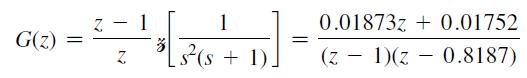
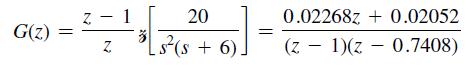
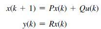
Consider the block diagram of a robot-arm control system shown in Fig. P8.6-4. This system is described in Problem 1.5-4. Let \(T=0.1\). It was shown in Problem 4.3-8 that\[G(z)=\frac{z-1}{z} z\left[\frac{2}{s^{2}(0.5 s+1)}ight]=\frac{0.01873 z+0.01752}{(z-1)(z-0.8187)}\]The frequency response for
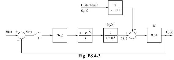
Consider the block diagram of an antenna control system shown in Fig. P8.6-5. Let T=0.05T=0.05 and the sensor gain be unity (H=1)(H=1).Extra \left or missing \rightThe frequency response for G(z)G(z).(a) Find the system phase margin with K=1K=1 and D(z)=1D(z)=1.(b) To reduce steady-state errors, KK
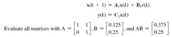
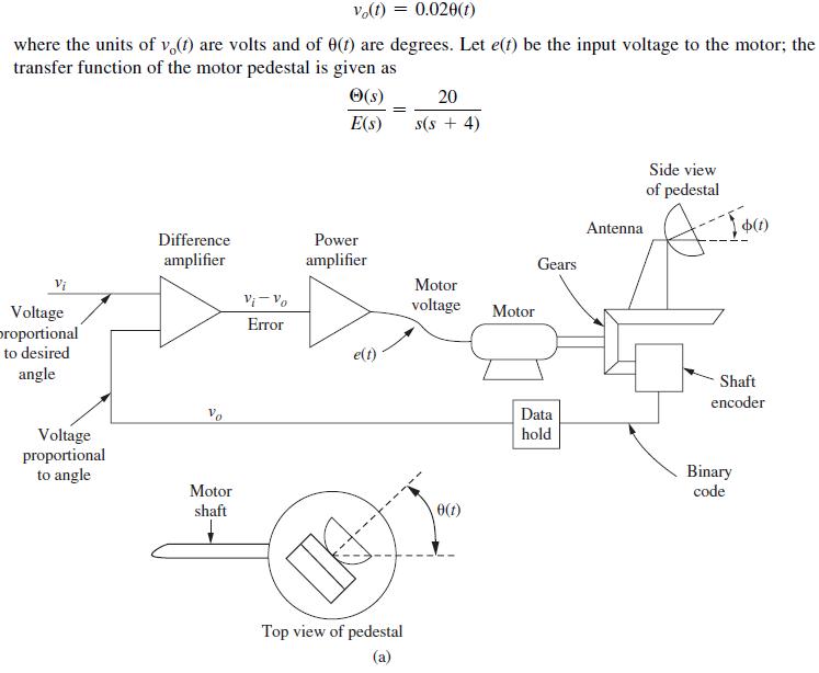
Consider the block diagram of a satellite control system shown in Fig. P8.6-6. This system is described in Problem 1.4-1. Let \(T=0.1 \mathrm{~s}, K=1, J=0.1\), and \(H_{k}=0.02\). It was shown in Problem 7.5-6 that\[G(z)=\frac{z-1}{z} z\left[\frac{10}{s^{3}}ight]=\frac{0.05(z+1)}{(z-1)^{2}}\]The
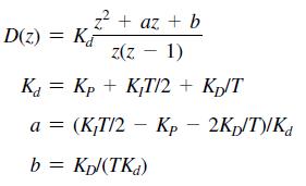
Write the difference equations required for the realization of the PID controller transfer function \(D(z)\) in (8-52). Let \({ }_{E(z)}\) be the controller input and \({ }_{M(z)}\) be the controller output.Equation 8-52 z + az + b z(z - 1) K = Kp + KT/2 + Kp/T a = (K;T/2 Kp2Kp/T)/Kd b = Kpl(TKd)
Showing 800 - 900
of 1058
1
2
3
4
5
6
7
8
9
10
11
Step by Step Answers
![It is shown in [6] that given the partitioned matrix H DE F G where each partition is nX n, the determinant](https://dsd5zvtm8ll6.cloudfront.net/images/question_images/1705/5/6/6/30465a8e0608f50a1705566303926.jpg)
![It is shown in [6] that given the partitioned matrix H = E F G where each partition is n X n, the](https://dsd5zvtm8ll6.cloudfront.net/images/question_images/1705/5/8/0/41365a9177d8f9bf1705580413336.jpg)

![(0.04)- 2 s(s+ 0.5)] = 0.04147 z - 0.7408 Note that the sensor gain is included in this transfer function.](https://dsd5zvtm8ll6.cloudfront.net/images/question_images/1705/6/4/1/20465aa04f44d6fc1705641202963.jpg)

![R(s) r(t) where x(k) is angular position and x2(k) is angular velocity. + x(k + 1) = = [61]8) + [0.25 (4) (a)](https://dsd5zvtm8ll6.cloudfront.net/images/question_images/1705/6/4/1/60665aa0686364641705641605084.jpg)
![R(s) E(S) T= 1 s D(z) 1-8-7's S M(s) Gp(s) 1 s+1] C(s)](https://dsd5zvtm8ll6.cloudfront.net/images/question_images/1705/4/8/8/16965a7af298dc5a1705488169103.jpg)
![10 2 (6 85 / (4) + / 3 /-(4) 0 0.5 x (k+ 1) = y (k)=[ 1 2 ]x (k)](https://dsd5zvtm8ll6.cloudfront.net/images/question_images/1705/4/0/4/57665a668a0620501705404574781.jpg)
![1 (* + 1) = [ 0 ] (*) + [ (*) 3 y (k)=[-2 1 ]x(k)](https://dsd5zvtm8ll6.cloudfront.net/images/question_images/1705/4/0/4/28365a6677b05d0c1705404282032.jpg)
![01 (+)-x(*)+-(*) 1) = 03 y(k)=[-2 1 ]x(*)](https://dsd5zvtm8ll6.cloudfront.net/images/question_images/1705/4/0/5/31365a66b81119601705405311527.jpg)
![where A x(k+ 1) = Ax(k) + Bu(k) y(k) = Cx(k) 0 -[-2-3] = B = -A C = [01]](https://dsd5zvtm8ll6.cloudfront.net/images/question_images/1705/6/4/3/65365aa0e8577d551705643651451.jpg)
![P(N + 1) = P(N) - P(N)f(N + 1) Y Y [ 1/2+ X + + F7(N + 1) = P(N)E(N + 1)] *'F*(N + 1) = P(N) a Y (10-56)](https://dsd5zvtm8ll6.cloudfront.net/images/question_images/1705/6/4/4/40765aa1177b13c91705644406586.jpg)
![y=[0; 1; 0.9; 0.71; 0.749; 0.7831; 0.7719]; u=ones (length (y), 1); T=0.1; % Create a data object using the](https://dsd5zvtm8ll6.cloudfront.net/images/question_images/1705/6/4/4/65365aa126d0f25f1705644651976.jpg)

![with the cost function x(k+ 1) = 0.6x(k) + 0.5u(k) 3 J3 = [2x(k) + 7u(k)] k = 0](https://dsd5zvtm8ll6.cloudfront.net/images/question_images/1705/6/4/5/66365aa165f427181705645662333.jpg)
![with A = 208 0 0 0 3 0 -8 -6 x = Ax + Bu y = Cx 0 B = 0, and C= [1 0 0]. Using = 8 0 0 0 6 0 0 4 3 R = 1.5](https://dsd5zvtm8ll6.cloudfront.net/images/question_images/1705/6/4/6/01865aa17c25a3141705646016987.jpg)
![with the cost function x(k+ 1) = Ax(k) + Bu(k) N JN = [Qx(k) + Ru(k)] k=0](https://dsd5zvtm8ll6.cloudfront.net/images/question_images/1705/6/4/6/40665aa1946d01db1705646405621.jpg)
![x(k + 1) [ = 0.999946 -0.177854E-1 y(k) [21]x(k) + v(k) 0.592847E 2] 0.976233 2xCA x(k) + [0.178567E 4](https://dsd5zvtm8ll6.cloudfront.net/images/question_images/1705/6/4/7/61065aa1dfa5ee561705647609045.jpg)
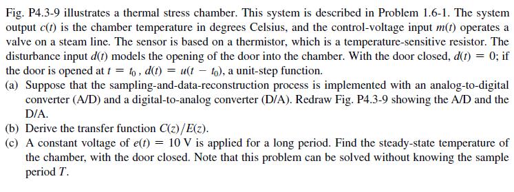
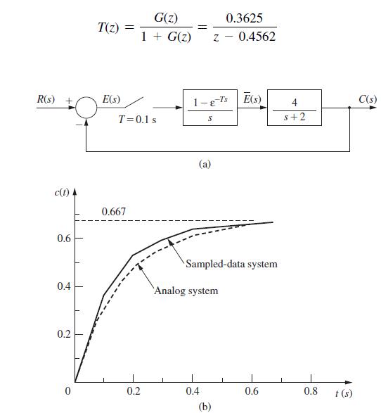
![where G(2) is defined as C(z) = G(z) 1 + G(z) -R(z) -Ts G(z) 0 = [1-8,4] - - 1 = S s +2 ss 4 +2)](https://dsd5zvtm8ll6.cloudfront.net/images/question_images/1705/6/5/1/99565aa2f1b87d7c1705651993885.jpg)
![R(s) m(kT) = e(kT) - 0.9e[(k 1)T] + m[(k 1)T] Gp(s) 1 s+1 T= 1 s D(z) 1-8-7's S M(s) Figure P6.5-2 System](https://dsd5zvtm8ll6.cloudfront.net/images/question_images/1705/5/6/0/64965a8ca49e2c881705560649848.jpg)