New Semester
Started
Get
50% OFF
Study Help!
--h --m --s
Claim Now
Question Answers
Textbooks
Find textbooks, questions and answers
Oops, something went wrong!
Change your search query and then try again
S
Books
FREE
Study Help
Expert Questions
Accounting
General Management
Mathematics
Finance
Organizational Behaviour
Law
Physics
Operating System
Management Leadership
Sociology
Programming
Marketing
Database
Computer Network
Economics
Textbooks Solutions
Accounting
Managerial Accounting
Management Leadership
Cost Accounting
Statistics
Business Law
Corporate Finance
Finance
Economics
Auditing
Tutors
Online Tutors
Find a Tutor
Hire a Tutor
Become a Tutor
AI Tutor
AI Study Planner
NEW
Sell Books
Search
Search
Sign In
Register
study help
computer science
digital control system analysis and design
Digital Signal Processing System Analysis And Design 2nd Edition Paulo S. R. Diniz, Eduardo A. B. Da Silva , Sergio L. Netto - Solutions
Design a highpass filter satisfying the specification below using the frequency sampling method:\[\begin{aligned}M & =40 \\\Omega_{\mathrm{r}} & =1.0 \mathrm{rad} / \mathrm{s} \\\Omega_{\mathrm{p}} & =1.5 \mathrm{rad} / \mathrm{s} \\\Omega_{\mathrm{s}} & =5.0 \mathrm{rad} / \mathrm{s}
Plot and compare the characteristics of the Hamming window and the corresponding magnitude response for \(M=5,10,15,20\).
Plot and compare the rectangular, triangular, Bartlett, Hamming, Hann, and Blackman window functions and the corresponding magnitude responses for \(M=20\).
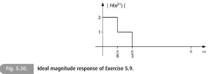
Determine the ideal impulse response associated with the magnitude response shown in Figure 5.30, and compute the corresponding practical filter of orders \(M=10,20,30\) using the Hamming window. 4 | H(el) | 2 3 Fig. 5.30. Ideal magnitude response of Exercise 5.9. FR 3
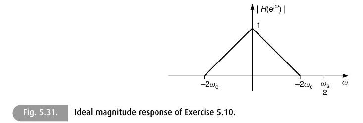
For the magnitude response shown in Figure 5.31, where \(\omega_{\mathrm{s}}=2 \pi\) denotes the sampling frequency:(a) Determine the ideal impulse response associated with it.(b) Design a fourth-order FIR filter using the triangular window with \(\omega_{\mathrm{c}}=\frac{\pi}{4}\). | H(e) | 1
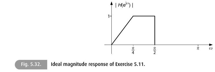
For the magnitude response shown in Figure 5.32:(a) Determine the ideal impulse response associated with it.(b) Design a fourth-order FIR filter using the Hann window. Fig. 5.32. 1- | H(ejo) | B| 4 Ideal magnitude response of Exercise 5.11. 2 -B
Design a bandpass filter satisfying the specification below using the Hamming, Hann, and Blackman windows:\[\begin{aligned}M & =10 \\\Omega_{\mathrm{c}_{1}} & =1.125 \mathrm{rad} / \mathrm{s}\\\Omega_{\mathrm{c}_{2}} & =2.5 \mathrm{rad} / \mathrm{s} \\\Omega_{\mathrm{s}} & =10 \mathrm{rad} /
Plot and compare the characteristics of the Kaiser window function and corresponding magnitude response for \(M=20\) and different values of \(\beta\).
Design the following filters using the Kaiser window:(a) \(A_{\mathrm{p}}=1.0 \mathrm{~dB}\)\(A_{\mathrm{r}}=40 \mathrm{~dB}\)\(\Omega_{\mathrm{p}}=1000 \mathrm{rad} / \mathrm{s}\)\(\Omega_{\mathrm{r}}=1200 \mathrm{rad} / \mathrm{s}\)\(\Omega_{\mathrm{s}}=5000 \mathrm{rad} / \mathrm{s}\).(b)
Determine a complete procedure for designing differentiators using the Kaiser window.
Repeat Exercise 5.14(a) using the Dolph-Chebyshev window. Compare the transition bandwidths and the stopband attenuation levels for the two resulting filters.Exercise 5.14(a)(a) \(A_{\mathrm{p}}=1.0 \mathrm{~dB}\)\(A_{\mathrm{r}}=40 \mathrm{~dB}\)\(\Omega_{\mathrm{p}}=1000 \mathrm{rad} /
Design a maximally flat lowpass filter satisfying the specification below:\[\begin{aligned}& \omega_{\mathrm{c}}=0.4 \pi \mathrm{rad} / \mathrm{sample} \\& T_{\mathrm{r}}=0.2 \pi \mathrm{rad} / \mathrm{sample}\end{aligned}\]where \(T_{\mathrm{r}}\) is the transition band as defined in Section 5.5.
Design three narrowband filters, centered on the frequencies \(770 \mathrm{~Hz}, 852 \mathrm{~Hz}\), and 941\(\mathrm{Hz}\), satisfying the specification below, using the minimax approach:\[\begin{aligned}& M=98 \\& \Omega_{\mathrm{s}}=2 \pi \times 5 \mathrm{kHz}\end{aligned}\]
Design Hilbert transformers of orders \(M=38,68\), and 98 using a Type IV structure and the Hamming window method.
Design a Hilbert transformer of order \(M=98\) using a Type IV structure and the triangular, Hann, and Blackman window methods.
Design a Hilbert transformer of order \(M=98\) using a Type IV structure and the Chebyshev method, and compare your results with those from Exercise 5.22.Exercise 5.22.Design a Hilbert transformer of order \(M=98\) using a Type IV structure and the triangular, Hann, and Blackman window methods.
Determine the output of the Hilbert transformer designed in Exercise 5.23 to the input signal \(\mathrm{x}\) determined as Fs \(=1500 ; \mathrm{TS}=1 / \mathrm{Fs} ; \mathrm{t}=0: \mathrm{TS}: 1-\mathrm{TS} ;\)\(\mathrm{fc} 1=200 ; \mathrm{fc} 2=300 ;\)\(\mathrm{x}=\cos \left(2^{*} \mathrm{pi}{
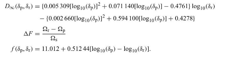
The following relationship estimates the order of a lowpass filter designed with the minimax approach (Rabiner et al., 1975). Design a series of lowpass filters and verify the validity of this estimate ( \(\Omega_{\mathrm{s}}\) is the sampling frequency):\[M \approx
Repeat Exercise 5.25 with the following order estimate (Kaiser, 1974):\[M \approx \frac{-20 \log _{10}\left(\sqrt{\delta_{\mathrm{p}} \delta_{\mathrm{r}}}\right)-13}{2.3237\left(\omega_{\mathrm{r}}-\omega_{\mathrm{p}}\right)}+1\]where \(\omega_{\mathrm{p}}\) and \(\omega_{\mathrm{r}}\) are the
Perform the algebraic design of a highpass FIR filter such that\[\begin{aligned}\omega_{\mathrm{p}} & =\frac{\omega_{\mathrm{s}}}{8}\\\delta_{\mathrm{p}} & =8 \delta_{\mathrm{r}}\end{aligned}\]using the WLS algorithm with a frequency grid of only two points.
Design a bandpass filter satisfying the specification below using the WLS and Chebyshev methods. Discuss the trade-off between the stopband minimum attenuation and total stopband energy when using the WLS-Chebyshev scheme.\[\begin{aligned}M & =50 \\\Omega_{\mathrm{r}_{1}} & =100 \mathrm{rad} /
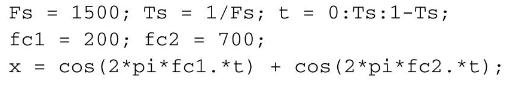
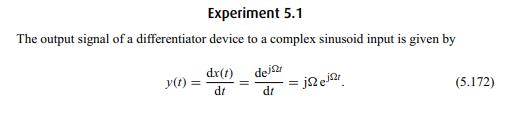
Repeat Experiment 5.1 with an input signal defined asand compare the results obtained with each differentiator system, by verifying what happens with each sinusoidal component in \(\mathrm{x}\). Fs 1500; Ts = 1/Fs; t = 0: Ts: 1-Ts; fc1 = 200; fc2 = 700; x = cos (2*pi*fc1. *t) + cos (2*pi* fc2. *t);
Change the values of Fs, total time length, and \(f_{C}\) in Experiment 5.1, one parameter at a time, and verify their individual influences on the output signal yielded by a differentiator system. Validate your analyses by differentiating the signal \(\mathrm{x}\) in Experiment 5.1 using the
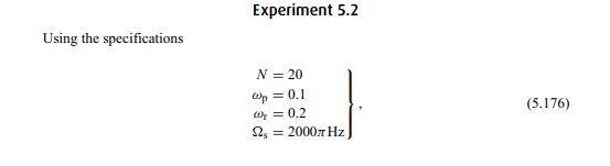
Change the filter specifications in Experiment 5.2, designing the filter accordingly, using the firpm command. Analyze the resulting magnitude response and the output signal to the input \(\mathrm{x}\) as defined in Experiment 1.3. Experiment 5.2 Using the specifications N = 20 wp = 0.1 W = 0.2
Determine the normalized specifications for the analog, lowpass, Chebysev filter corresponding to the highpass filter:\[\begin{aligned}A_{\mathrm{p}} & =0.2 \mathrm{~dB} \\A_{\mathrm{r}} & =50 \mathrm{~dB} \\\Omega_{\mathrm{r}} & =400 \mathrm{~Hz} \\\Omega_{\mathrm{p}} & =440
Determine the normalized specifications for the analog, lowpass, elliptic filter corresponding to the bandpass filter:\[\begin{aligned}A_{\mathrm{p}} & =2 \mathrm{~dB} \\A_{\mathrm{r}} & =40 \mathrm{~dB} \\\Omega_{\mathrm{r}_{1}} & =400 \mathrm{~Hz} \\\Omega_{\mathrm{p}_{1}} & =500 \mathrm{~Hz}
Design an analog elliptic filter satisfying the following specifications:\[\begin{aligned}A_{\mathrm{p}} & =1.0 \mathrm{~dB} \\A_{\mathrm{r}} & =40 \mathrm{~dB} \\\Omega_{\mathrm{p}} & =1000 \mathrm{~Hz} \\\Omega_{\mathrm{r}} & =1209 \mathrm{~Hz} .\end{aligned}\]
Design a lowpass Butterworth filter satisfying the following specifications:\[\begin{aligned}A_{\mathrm{p}} & =0.5 \mathrm{~dB} \\A_{\mathrm{r}} & =40 \mathrm{~dB} \\\Omega_{\mathrm{p}} & =100 \mathrm{~Hz} \\\Omega_{\mathrm{r}} & =150 \mathrm{~Hz} \\\Omega_{\mathrm{s}} & =500 \mathrm{~Hz}
Design a bandstop elliptic filter satisfying the following specifications:\[\begin{aligned}A_{\mathrm{p}} & =0.5 \mathrm{~dB} \\A_{\mathrm{r}} & =60 \mathrm{~dB} \\\Omega_{\mathrm{p}_{1}} & =40 \mathrm{~Hz} \\\Omega_{\mathrm{r}_{1}} & =50 \mathrm{~Hz} \\\Omega_{\mathrm{r}_{2}} & =70 \mathrm{~Hz}
Design highpass Butterworth, Chebyshev, and elliptic filters that satisfy the following specifications:\[\begin{aligned}A_{\mathrm{p}} & =1.0 \mathrm{~dB} \\A_{\mathrm{r}} & =40 \mathrm{~dB} \\\Omega_{\mathrm{r}} & =5912.5 \mathrm{rad} / \mathrm{s} \\\Omega_{\mathrm{p}} & =7539.8 \mathrm{rad} /
Design three bandpass digital filters, one with a central frequency of \(770 \mathrm{~Hz}\), a second of \(852 \mathrm{~Hz}\), and a third of \(941 \mathrm{~Hz}\). For the first filter, the stopband edges are at frequencies 697 and \(852 \mathrm{~Hz}\). For the second filter, the stopband edges are
Plot the zero-pole constellation for the three filters designed in Exercise 6.7 and visualize the resulting magnitude response in each case.Exercise 6.7Design three bandpass digital filters, one with a central frequency of \(770 \mathrm{~Hz}\), a second of \(852 \mathrm{~Hz}\), and a third of \(941
Create an input signal composed of three sinusoidal components of frequencies 770 \(\mathrm{Hz}, 852 \mathrm{~Hz}\), and \(941 \mathrm{~Hz}\), in MATLAB with \(\Omega_{\mathrm{s}}=8 \mathrm{kHz}\). Use the three filters designed in Exercise 6.7 to isolate each component in a different
The transfer function\[H(s)=\frac{\kappa}{\left(s^{2}+1.4256 s+1.23313\right)(s+0.6265)}\]corresponds to a lowpass normalized Chebyshev filter with passband ripple \(A_{\mathrm{p}}=0.5\) \(\mathrm{dB}\).(a) Determine \(\kappa\) such that the filter gain at DC is 1 .(b) Design a highpass digital
Transform the continuous-time highpass transfer function given by\[H(s)=\frac{s^{2}}{s^{2}+s+1}\]into a discrete-time transfer function using the impulse-invariance transformation method with \(\Omega_{\mathrm{s}}=10 \mathrm{rad} / \mathrm{s}\). Plot the resulting analog and digital magnitude
Repeat Exercise 6.11 using the bilinear transformation method and compare results from both exercises.Exercise 6.11Transform the continuous-time highpass transfer function given by\[H(s)=\frac{s^{2}}{s^{2}+s+1}\]into a discrete-time transfer function using the impulse-invariance transformation
Given the analog transfer function\[H(s)=\frac{1}{\left(s^{2}+0.76722 s+1.33863\right)(s+0.76722)},\]design transfer functions corresponding to discrete-time filters using both the impulseinvariance method and the bilinear transformation. Choose \(\Omega_{\mathrm{s}}=12 \mathrm{rad} / \mathrm{s}\).
Repeat Exercise 6.13 using \(\Omega_{\mathrm{s}}=24 \mathrm{rad} / \mathrm{s}\) and compare the results achieved in each case.Exercise 6.13Given the analog transfer function\[H(s)=\frac{1}{\left(s^{2}+0.76722 s+1.33863\right)(s+0.76722)},\]design transfer functions corresponding to discrete-time
Repeat Exercise 6.13 using MATLAB commands impinvar and bilinear.Exercise 6.13Given the analog transfer function\[H(s)=\frac{1}{\left(s^{2}+0.76722 s+1.33863\right)(s+0.76722)},\]design transfer functions corresponding to discrete-time filters using both the impulseinvariance method and the
Determine the original analog transfer function corresponding to\[H(z)=\frac{4 z}{z-\mathrm{e}^{-0.4}}-\frac{z}{z-\mathrm{e}^{-0.8}}\]assuming that the following method was employed in the analog to discrete-time mapping, with \(T=4\) :(a) Impulse invariance method.(b) Bilinear transformation
Determine the original analog transfer function corresponding to\[H(z)=\frac{2 z^{2}-\left(\mathrm{e}^{-0.2}+\mathrm{e}^{-0.4}\right) z}{\left(z-\mathrm{e}^{-0.2}\right)\left(z-\mathrm{e}^{0.4}\right)}\]assuming that the following method was employed in the analog to discrete-time mapping, with
This exercise describes the inverse Chebyshev approximation. The attenuation function of a lowpass inverse Chebyshev filter is characterized as\[\begin{aligned}\left|A\left(\mathrm{j} \Omega^{\prime}\right)\right|^{2} & =1+E\left(\mathrm{j} \Omega^{\prime}\right) E\left(-\mathrm{j}
Show that the lowpass-to-bandpass and lowpass-to-bandstop transformations proposed in Section 6.4 are valid.Section 6.4 Usually, in the approximation of a continuous-time filter, we begin by designing a nor- malized lowpass filter and then, through a frequency transformation, the filter with the
Apply the lowpass-to-highpass transformation to the filter designed in Exercise 6.4 and plot the resulting magnitude response.Exercise 6.4Design a lowpass Butterworth filter satisfying the following specifications:\[\begin{aligned}A_{\mathrm{p}} & =0.5 \mathrm{~dB} \\A_{\mathrm{r}} & =40
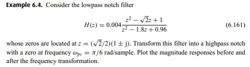
Revisit Example 6.4, now forcing the highpass zero at \(\omega_{\mathrm{p}_{1}}=2 \pi / 3\). Plot the magnitude responses before and after the transformation. Example 6.4. Consider the lowpass notch filter z22z+1 H(2) 0.004- 2-1.8z+0.96 (6.161) whose zeros are located at z = (2/2)(1 + j). Transform
Given the transfer function\[H(z)=0.06 \frac{z^{2}+\sqrt{2} z+1}{z^{2}-1.18 z+0.94}\]describe a frequency transformation to a bandpass filter with zeros at \(\pi / 6\) and \(2 \pi / 3\).
Design a phase equalizer for the elliptic filter of Exercise 6.6 with the same order as the filter.Exercise 6.6Design highpass Butterworth, Chebyshev, and elliptic filters that satisfy the following specifications:\[\begin{aligned}A_{\mathrm{p}} & =1.0 \mathrm{~dB} \\A_{\mathrm{r}} & =40
Design a lowpass filter satisfying the following specifications:\[\begin{aligned}M(\Omega T)=1.0, & \text { for } 0.0 \Omega_{\mathrm{s}}
The desired impulse response for a filter is given by \(g(n)=1 / 2^{n}\). Design a recursive filter such that its impulse response \(h(n)\) equals \(g(n)\) for \(n=0,1, \ldots, 5\).
Plot and compare the magnitude responses associated with the ideal and approximated impulse responses in Exercise 6.26.Exercise 6.26.The desired impulse response for a filter is given by \(g(n)=1 / 2^{n}\). Design a recursive filter such that its impulse response \(h(n)\) equals \(g(n)\) for
Design a filter with 10 coefficients such that its impulse response approximates the following sequence:\[g_{n}=\left(\frac{1}{6^{n}}+10^{-n}+\frac{0.05}{n+2}\right) u(n)\]Choose a few key values for \(M\) and \(N\), and discuss which choice leads to the smallest mean-squared error after the tenth
Compare the magnitude responses associated with the filters designed in Exercise 6.28 for several values of \(M\) and \(N\).Exercise 6.28Design a filter with 10 coefficients such that its impulse response approximates the following
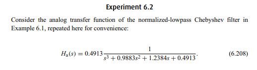
Repeat Experiment 6.2 using \(F_{\mathrm{s}}=10 \mathrm{~Hz}\). Compare the magnitude response of the resulting discrete-time transfer function with the one obtained in the experiment. Experiment 6.2 Consider the analog transfer function of the normalized-lowpass Chebyshev filter in Example 6.1,
Determine the Pascal matrix \(\mathbf{P}_{N+1}\) defined in Experiment 6.2 for \(N=4\) and \(N=5\). Experiment 6.2 Consider the analog transfer function of the normalized-lowpass Chebyshev filter in Example 6.1, repeated here for convenience: 1 Ha(s) 0.4913 (6.208) s3+0.9883s2+1.2384s +0.49131
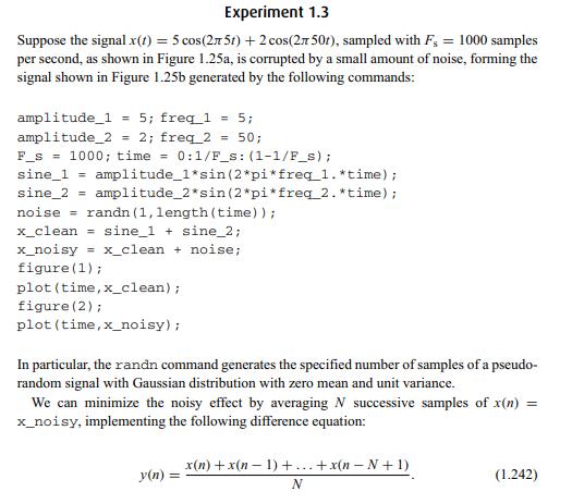
Design an IIR digital filter to reduce the amount of noise in the two sinusoidal components in Experiment 1.3. Evaluate your specifications by processing x_noisy, as defined in that experiment, with the designed filter and verifying the output signal-to-noise ratio. Experiment 1.3 Suppose the
Use the periodogram algorithm to estimate the PSD of a length- \(L\) white-noise sequence generated by the MATLAB command randn. Average your results for \(N\) realizations of the white noise and verify the influences of \(L\) and \(N\) on the resulting estimate.
Use the periodogram algorithm to estimate the PSD of \(L=1024\) samples of the following signal:\[x(n)=\cos \frac{2 \pi}{20} n+x_{1}(n)\]where\[x_{1}(n)=-0.9 x_{1}(n-1)+x_{2}(n),\]where \(x_{2}(n)\) is a white Gaussian noise with variance \(\sigma_{X_{2}}^{2}=0.19\).
Use the periodogram algorithm to estimate the PSD of the following signal:\[x(n)=\cos \frac{2 \pi}{4} n+x_{1}(n)\]where\[x_{1}(n)=-0.9 x_{1}(n-1)+x_{2}(n) \text {, }\]where \(x_{2}(n)\) is a white Gaussian noise with variance \(\sigma_{X_{2}}^{2}=0.19\). Use in this case \(L=512, L=1024\), and
An AR process is generated by applying white Gaussian noise, with variance \(\sigma_{X}^{2}\), to a first-order filter with transfer function\[H(z)=\frac{z}{z-a} .\]This process has the autocorrelation matrix\[\mathbf{R}_{Y}=\frac{\sigma_{X}^{2}}{1-a^{2}}\left[\begin{array}{cccc}1 & a & \cdots &
In Exercise 7.4, consider \(a=0.8\) and plot the minimum-variance solution for window lengths equal to \(L=4, L=10\), and \(L=50\). Compare the estimated PSD in each case with the actual PSD and comment on the results.Exercise 7.4An AR process is generated by applying white Gaussian noise, with
Use the minimum-variance method to estimate the PSD of \(L=256\) samples of the following signal:\[y(n)=\sin \frac{\pi}{2} n+x_{1}(n)\]where\[x_{1}(n)=-0.8 x_{1}(n-1)+x_{2}(n) \text {, }\]with \(x_{2}(n)\) being a white Gaussian noise with variance \(\sigma_{X_{2}}^{2}=0.36\).
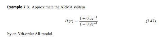
(a) Use the MATLAB command roots to determine the pole locations of the AR approximation, using \(N=1,2,3,4\), for the ARMA system given in Example 7.3.(b) Find the AR impulse response for each value of \(N\) in the previous item and compare your results with the impulse response of the original
Find an \(N\) th-order AR approximation for the ARMA system\[H(z)=\frac{1-1.5 z^{-1}}{1+0.5 z^{-1}}\]and compare the resulting magnitude response to the original ARMA system. Observe that in this case the ARMA system presents a zero outside the unit circle.
Given two first-order AR processes generated by the same zero-mean white noise with unit variance whose respective poles are located at \(a_{1}\) and \(-a_{1}\), with \(\left|a_{1}\right|
Find an \(N\) th-order AR approximation for the ARMA system\[H(z)=\frac{\left(1-0.8 z^{-1}\right)\left(1-0.9 z^{-1}\right)}{\left(1-0.5 z^{-1}\right)\left(1+0.5 z^{-1}\right)}\]and compare the resulting magnitude response with the original ARMA system.
(a) Find an \(M\) th-order MA approximation for the ARMA system given in Example 7.3.(b) Use the roots command in MATLAB to determine the zero locations of the MA approximation for \(M=1,2,3,4\).(c) Find the MA impulse response for each value of \(M\) and compare your results with the impulse
Show that, for a causal AR system with a zero-mean input \(x(n)\) and output \(y(n)\) :\[E\{x(n) y(n-v)\}= \begin{cases}\sigma_{X}^{2}, & \text { for } v=0 \\ 0, & \text { for } v>0\end{cases}\]
Solve the Yule-Walker equations for a second-order AR system\[H(z)=\frac{1}{1+a_{1} z^{-1}+a_{2} z^{-2}}\]determining \(R_{Y}(v)\) for a white-noise input of variance \(\sigma_{X}^{2}\).
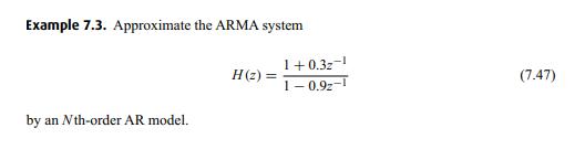
Solve the Yule-Walker equations provided by Equation (7.58) for the ARMA system given in Example 7.3, assuming a unit-variance white-noise input. Example 7.3. Approximate the ARMA system by an Nth-order AR model. 1+0.32 H(z) = (7.47) 1 0.92
Determine the second-order optimal predictor in the minimum MSE sense for the output process of an MA system\[H(z)=1+2 z^{-1}+3 z^{-2}\]to a unit-variance white-noise input.
Show that the autocorrelation method yields an AR system whose poles are not outside the unit circle in the \(z\) plane.
Show, by a simple numerical example, that the covariance method may yield an AR system with poles outside the unit circle in the \(z\) plane.
Given two first-order AR processes, generated by the same zero-mean white noise with unit variance, whose respective poles are located at \(z=0.8\) and \(z=-0.8\), generate a new process by adding the outcomes of these AR processes. Estimate the fourth-order AR model for the resulting process using
Given an MA process generated by applying a zero-mean white noise with unit variance to a system described by\[H(z)=0.921-1.6252 z^{-1}+z^{-2} \text {, }\]estimate the third-order AR model for the resulting process using the linear prediction method and comment on the results.
Use the covariance method to estimate the PSD of \(L=1024\) samples for the following signal:\[x(n)=\cos \frac{2 \pi}{L} n+x_{1}(n)\]where \[x_{1}(n)=a x_{1}(n-1)+x_{2}(n),\]with \(x_{2}(n)\) being a white Gaussian noise with variance \(1-a^{2}\).(a) Choose \(a=-0.9\) and \(N=4\).(b) Choose
Estimate the PSD of the signal\[x(n)=\mathrm{e}^{\mathrm{j}(2 \pi / 8) n}+x_{1}(n)\]with \(x_{1}(n)\) being a white Gaussian noise with unit variance.
Solve Exercise 7.21 by estimating the AR parameters using the autocorrelation method.Exercise 7.21Use the covariance method to estimate the PSD of \(L=1024\) samples for the following signal:\[x(n)=\cos \frac{2 \pi}{L} n+x_{1}(n)\]where \[x_{1}(n)=a x_{1}(n-1)+x_{2}(n),\]with \(x_{2}(n)\) being a
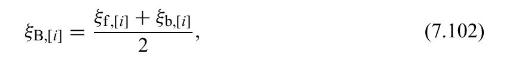
Verify that the Burg reflection coefficients, as given in Equation (7.108), determine the minimum value of \(\xi_{\mathrm{B},[i]}\) defined in Equation (7.102). SB,[i] = f,[i] + $b[i] 2 (7.102)
Solve Exercise 7.21 by estimating the AR parameters using the Levinson-Durbin recursions with the Burg reflection coefficients.Exercise 7.21Use the covariance method to estimate the PSD of \(L=1024\) samples for the following signal:\[x(n)=\cos \frac{2 \pi}{L} n+x_{1}(n)\]where \[x_{1}(n)=a
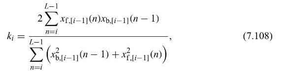
Show that the Burg reflection coefficients provided in Equation (7.108) are such that \(\left|k_{i}\right| ki = L-1 2x [i-1] (n)xb[i-1](n - 1) L-1 n=i (x-11(n-1)+x-11(n)) n=i (7.108)
Determine closed-form expressions for the Levinson-Durbin reflection coefficients \(k_{1}, k_{2}\), and \(k_{3}\) as functions of \(R_{Y}(v)\).
Estimate the PSD of the ARMA system output in Exercise 7.11 to a unit-variance white-noise input. Use the standard periodogram method and the autocorrelation method with \(N=1,2,3,4\) and compare the results in each case.Exercise 7.11Find an \(N\) th-order AR approximation for the ARMA
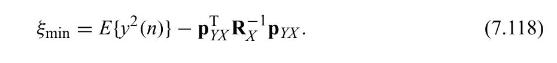
Show that the minimum MSE value achieved by the Wiener solution is given by Equation (7.118). Emin = E{y (n)} - px RX Pxx (7.118)
A random process \(x(n)\) is generated by applying a white noise \(w(n)\) with unit variance as input to a system described by the following transfer function:\[H(z)=\frac{1}{z^{2}-0.36}\]Compute the second-order Wiener filter that relates \(x(n)\) to the output \(y(n)\) of the
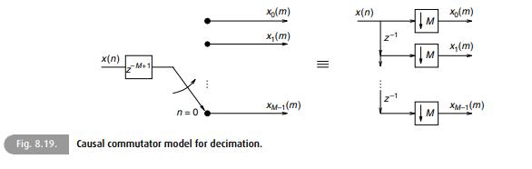
Deduce the two noble identities (Equations (8.30) and (8.31)) using an argument in the time domain. DMX (2))H(z) = DM{X (2)H(z)}, (8.30)
Prove Equations (8.28) and (8.29). x (mM/L), {x m-N, k Z y(m) = 10. m=kL, k Z otherwise (8.28)
The sequence\[x=0.125,0.25,0.5,1,2,4\]is filtered by a filter with transfer function\[H(z)=\frac{1}{3}\left(1+z^{-1}+z^{-2}\right)\]and the result is decimated by 2 . The output is then upsampled by 2 and filtered by the same \(H(z)\). Generate the resulting sequence and interpret the results.
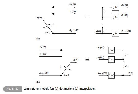
Show that decimation is a time-varying, but periodically time-invariant, operation and that interpolation is a time-invariant operation.
Design two interpolation filters, one lowpass and the other multiband (Equation (8.22)), with specifications\[\begin{aligned}& \delta_{\mathrm{p}}=0.0002 \\& \delta_{\mathrm{r}}=0.0001 \\& \Omega_{\mathrm{s}}=10000 \mathrm{rad} / \mathrm{s} \\& L=10\end{aligned}\]Assume that we are
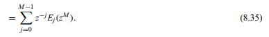
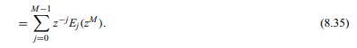
Show the polyphase decomposition structure, as given in Equation (8.35), for an FIR filter with impulse response\[h(n)=0.25,0.5,0.5,1,1,0.5,0.5,0.25\]for \(n=0,1, \ldots, 7\). Try to minimize the number of multiplications. M-1 =E(2M). j=0 (8.35)
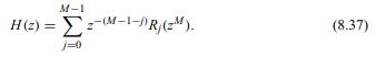
Show the polyphase decomposition structure, as given in Equation (8.37), for an FIR filter with impulse response\[h(n)=-0.375,0.25,-0.5,1,-1,0.5,-0.25,0.375\]for \(n=0,1, \ldots, 7\). Try to minimize the number of multiplications. M-I H(2)=(M-1-DR(ZM). J=0 (8.37)
Show the polyphase decomposition structures, as given in Equations (8.35) and (8.37), for an FIR filter with impulse response\[h(n)=a,b, c,d, e,-d,-c,-b,-a\]for \(n=0,1, \ldots, 8\), minimizing the number of multiplications. M-1 ==E(z). j=0 (8.35)
Show that the zeroth polyphase component of an \(L\) th band filter is constant in the frequency domain.
Prove that for a linear-phase filter whose impulse response has length \(M L\), its \(M\) polyphase components (Equation (8.35)) should satisfy\[E_{j}(z)= \pm z^{-(L-1)} E_{M-1-j}\left(z^{-1}\right) .\] M-1 ==E(z). j=0 (8.35)
Design a lowpass filter using one decimation/interpolation stage satisfying the following specifications:\[\begin{aligned}& \delta_{\mathrm{p}}=0.001 \\& \delta_{\mathrm{r}} \leq 0.0001 \\& \Omega_{\mathrm{p}}=0.01 \Omega_{\mathrm{s}} \\& \Omega_{\mathrm{r}}=0.02 \Omega_{\mathrm{s}} \\&
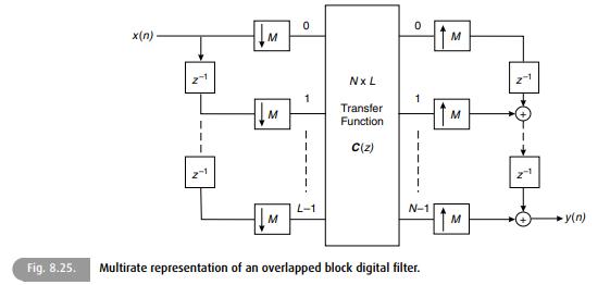
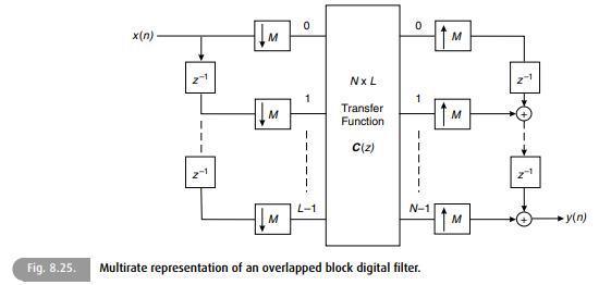
In the serial-to-parallel converter of Figure 8.25, see also Figure 8.19, assume \(M=2\) and \(L=3\) and that the input signal is a sequence given by\[x(n)=0,0,a, b,c, d,e, f, g, h, i, 0,0\]for \(n=0,1, \ldots, 12\). Determine the output sequences. 0 0 x(n) M M Nx L 1 Transfer M M Function I 1 C(z)
In the parallel-to-serial converter of Figure 8.25, see also Figure 8.18, assume \(M=2\) and \(N=3\) and that the input signals are given by\[\begin{aligned}& x_{1}(n)=0,0, a \\& x_{2}(n)=b,c, d \\& x_{3}(n)=e,f, g \\& x_{4}(n)=h, i, 0 .\end{aligned}\]Determine the output sequence.
In Exercise 8.7, a nonminimum delay overlapped solution is possible by choosing\[\mathbf{C}_{l}(z)=\left[\begin{array}{cccc}D_{0}(z) & R_{1}(z) & 0 & 0 \\0 & R_{0}(z) & R_{1}(z) & 0 \\0 & 0 & R_{0}(z) & D_{1}(z)\end{array}\right]\]Derive the corresponding
Given the matrix\[\mathbf{C}(z)=\left[\begin{array}{ccc}R_{0}(z) & R_{1}(z) & R_{2}(z) \\z^{-1} R_{2}(z) & R_{0}(z) & R_{1}(z) \\z^{-1} R_{1}(z) & z^{-1} R_{2}(z) & R_{0}(z)\end{array}\right]\]verify if \(\mathbf{C}^{2}(z)\) is pseudo-circulant.
Given the matrix\[\mathbf{C}(z)=\left[\begin{array}{cc}R_{0}(z) & R_{1}(z) \\z^{-1} R_{1}(z) & R_{0}(z)\end{array}\right]\]show that its inverse is pseudo-circulant.
Showing 400 - 500
of 1058
1
2
3
4
5
6
7
8
9
10
11
Step by Step Answers