New Semester Started Get 50% OFF Study Help! --h --m --s Claim Now

Question Answers

Textbooks

Find textbooks, questions and answers

Oops, something went wrong!

Change your search query and then try again

Result Not Found

Books FREE
Study Help
Tutors
AI Study Planner NEW
Sell Books

Search
Sign In
Register

study help
engineering
modern control systems

Modern Control Systems 14th Global Edition Richard Dorf, Robert Bishop - Solutions

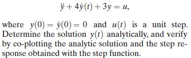
Consider the differential equation +4y(t)+3y= u, where y(0) = y(0) = 0 and u(t) is a unit step. Determine the solution y(t) analytically, and verify by co-plotting the analytic solution and the step re- sponse obtained with the step function.
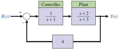
Consider the feedback system depicted in Figure CP2.2.(a) Compute the closed-loop transfer function using the series and feedback functions.(b) Obtain the closed-loop system unit step response with the step function, and verify that final value of the output is 0.571. Controller Plant 1 5+2 R(s)
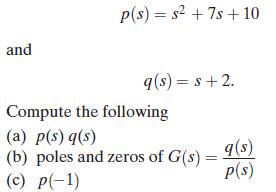
Consider the two polynomials and p(s) s+7s+10 9(s)=s+2. Compute the following (a) p(s) q(s) (b) poles and zeros of G(s) = q(s) (c) p(-1) P(s)
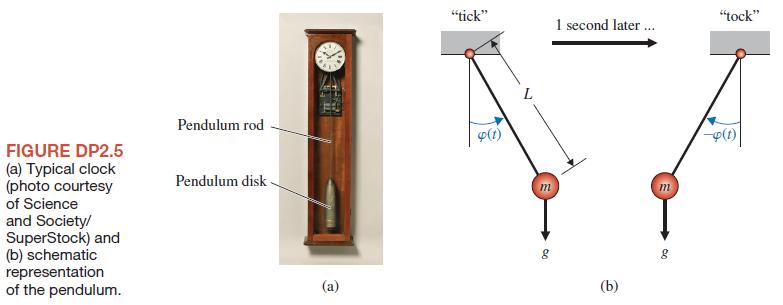
Consider the clock shown in Figure DP2.5. The pendulum rod of length L supports a pendulum disk.Assume that the pendulum rod is a massless rigid thin rod and the pendulum disc has mass m. Design the length of the pendulum, L, so that the period of motion is 2 seconds. Note that with a period of 2
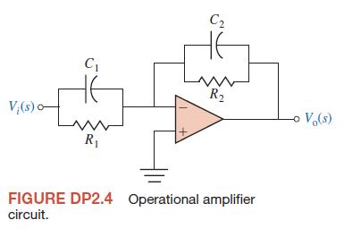
An operational amplifier circuit that can serve as an active low-pass filter circuit is shown in Figure DP2.4.Determine the transfer function of the circuit, assuming an ideal op-amp. Find υ0 (t) when the input isυ1 (t) = δ(t) , t ≥ 0. C C R V(s) o Vo(s) R FIGURE DP2.4 Operational amplifier
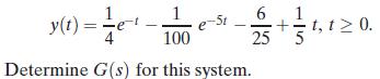
DP2.3 An input r(t) = t, t ≥ 0, is applied to a black box with a transfer function G(s). The resulting output response, when the initial conditions are zero, is y(t)=- 1 6 t,t20. 100 25 Determine G(s) for this system.
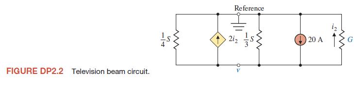
DP2.2 The television beam circuit of a television is represented by the model in Figure DP2.2. Select the unknown conductance G so that the voltage v is 24 V.Each conductance is given in siemens (S). FIGURE DP2.2 Television beam circuit.. + w Reference 13 212 3s 20 A ww G
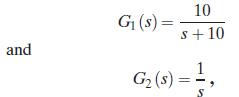
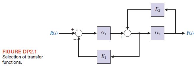
A control system is shown in Figure DP2.1. Withdetermine the gains K1 and K2 such that the final value y(t) as t S q reaches y S 1 and the closed-loop poles are located at s1= –20 and s2 = – 0.5. and G(s)= 10 s+10 = 1, G (5) =
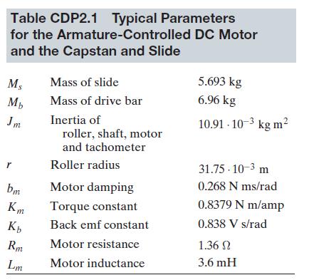
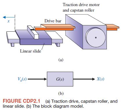
We want to accurately position a table for a machine as shown in Figure CDP2.1. A traction-drive motor with a capstan roller possesses several desirable characteristics compared to the more popular ball screw.The traction drive exhibits low friction and no backlash.However, it is susceptible to
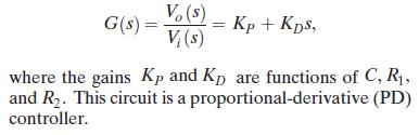
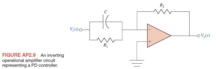
Consider the inverting operational amplifier in Figure AP2.9. Find the transfer function Vo (s)/Vi (s).Show that the transfer function can be expressed as V(s) G(s) = Kp + Kps, V(s) where the gains Kp and Kp are functions of C, R, and R2. This circuit is a proportional-derivative (PD) controller.
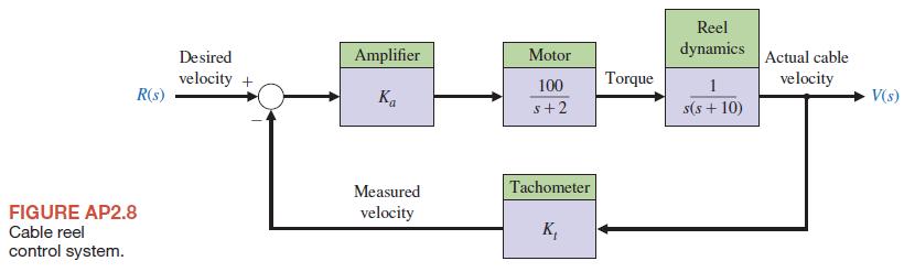
AP2.8 Consider the cable reel control system given in Figure AP2.8. Find the value of Kt and Ka such that the percent overshoot is P.O. ≤ 15% and a zero steady state error to a unit step is achieved. Compute the closed-loop response y(t) analytically and confirm that the steady-state response and
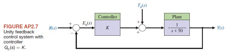
AP2.7 Consider the unity feedback system described in the block diagram in Figure AP2.7. Compute analytically the response of the system to an impulse disturbance.Determine a relationship between the gain K and the minimum time it takes the impulse disturbance response of the system to reach y(t)
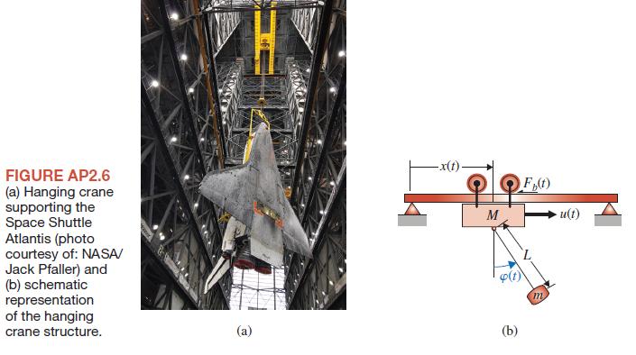
Consider the hanging crane structure in Figure AP2.6. Write the equations of motion describing the motion of the cart and the payload. The mass of the cart is M, the mass of the payload is m, the massless rigid connector has length L, and the friction is modeled as Fb (t) = −bx(t) where x(t) is
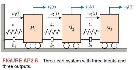
AP2.5 For the three-cart system (Figure AP2.5), obtain the equations of motion. The system has three inputs u1 (t), u2 (t), and u3 (t) and three outputs x1 (t), x2 (t), and x3 (t). Obtain three second-order ordinary differential equations with constant coefficients. If possible, write the equations
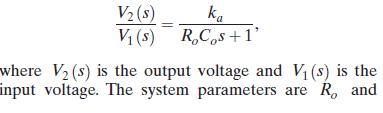
AP2.4 Consider a DC amplifier given byCo, the output resistance and capacitance, respectively.The DC amplifier is illustrated in Table 2.4. (a)Determine the response of the system to a unit step V1 (s) = 1/s. (b) As t → ∞, what value does the step response determined in part (a) approach? This
Consider the feedback control system in Figure AP2.3. Define the tracking error as E(s) = R(s)−Y(s).(a) Determine a suitable H(s) such that the tracking error is zero for any input R(s) in the absence of a disturbance input (that is, when Td (s) = 0). (b) Using H(s) determined in part (a),
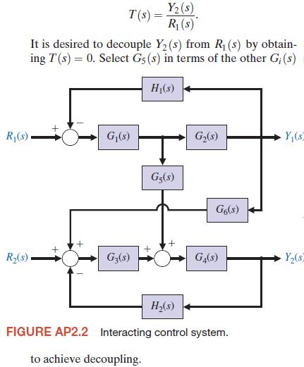
AP2.2 A system has a block diagram as shown in Figure AP2.2. Determine the transfer function Y2(s) T(s) = R(s) It is desired to decouple Y2(s) from R (s) by obtain- ing T(s) = 0. Select G5 (s) in terms of the other G;(s) H(s) R(s) G(s) G5(s) G(s) Y(s G6(s) R(s) G3(5) G4(s) Y(s H(s) FIGURE AP2.2
A first-order RL circuit consisting of a resistor and an inductor in series driven by a voltage source is one of the simplest analog infinite impulse response electronic filters. For an input voltage of 5 V, the current at t = 1 s is 2 A, and the steady state current is 5 A when t → ∞.
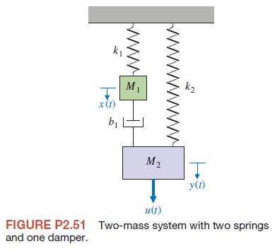
Consider the two-mass system in Figure P2.51.Find the set of differential equations describing the system. x(t) Mi k2 b M2 I y(t) u(t) FIGURE P2.51 Two-mass system with two springs and one damper.
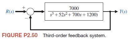
P2.50 A closed-loop control system is shown in Figure P2.50.(a) Determine the transfer function T(s) = Y(s)/R(s).(b) Determine the poles and zeros of T(s).(c) Use a unit step input, R(s) = 1/s, and obtain the partial fraction expansion for Y(s) and the value of the residues.(d) Plot y(t) and
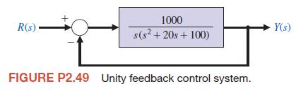
P2.49 A closed-loop control system is shown in Figure P2.49.(a) Determine the transfer function T(s) = Y(s)/R(s).(b) Determine the poles and zeros of T(s).(c) Use a unit step input, R(s) = 1/s, and obtain the partial fraction expansion for Y(s) and the value of the residues.(d) Plot y(t) and
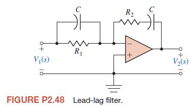
The circuit shown in Figure P2.48 is called a lead-lag filter.(a) Find the transfer function V2 (s)/V1 (s). Assume an ideal op-amp.(b) Determine V2 (s)/V1 (s) when R1 = 250 kΩ, R2 = 250 kΩ, C1 = 2 μF, and C2 = 0.3 μF.(c) Determine the partial fraction expansion for V2 (s)/V1 (s). V(s) C R www R
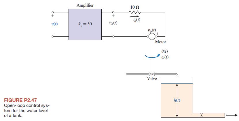
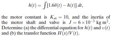
The water level h(t) in a tank is controlled by an open-loop system, as shown in Figure P2.47.A DC motor controlled by an armature current ia turns a shaft, opening a valve. The inductance of the DC motor is negligible, that is, La = 0. Also, the rotational friction of the motor shaft and valve is
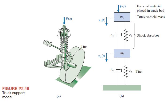
A load added to a truck results in a force F(s) on the support spring, and the tire flexes as shown in Figure P2.46(a). The model for the tire movement is shown in Figure P2.46(b). Determine the transfer function X1 (s)/F (s). FIGURE P2.46 Truck support model. F(s) x1(t) F(t) my Force of material
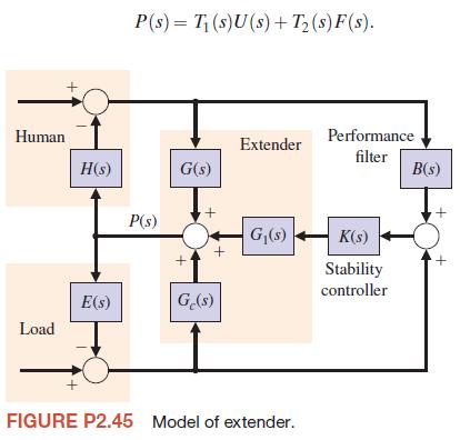
To exploit the strength advantage of robot manipulators and the intellectual advantage of humans, a class of manipulators called extenders has been examined [22]. The extender is defined as an active manipulator worn by a human to augment the human’s strength. The human provides an input U(s), as
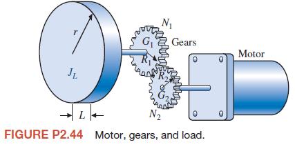
P2.44 An ideal set of gears is connected to a solid cylinder load as shown in Figure P2.44. The inertia of the motor shaft and gear G2 is Jm. Determine (a) the inertia of the load JL and (b) the torque T at the motor shaft.Assume the friction at the load is bL and the friction at the motor shaft is
An ideal set of gears is shown in Table 2.4, item 10.Neglect the inertia and friction of the gears and assume that the work done by one gear is equal to that of the other. Derive the relationships given in item 10 of Table 2.4. Also, determine the relationship between the torques Tm and TL.
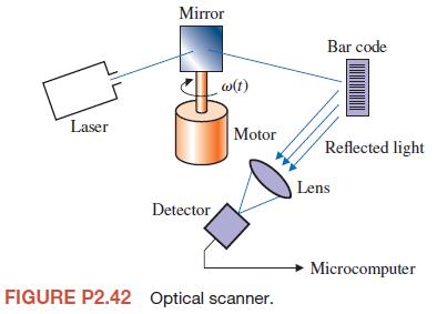
In many applications, such as reading product codes in supermarkets and in printing and manufacturing, an optical scanner is utilized to read codes, as shown in Figure P2.42. As the mirror rotates, a friction force is developed that is proportional to its angular speed. The friction constant is
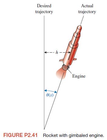
The lateral control of a rocket with a gimbaled engine is shown in Figure P2.41. The lateral deviation from the desired trajectory is h and the forward rocket speed is V. The control torque of the engine is Tc (s) and the disturbance torque is Td (s). Derive the describing equations of a linear
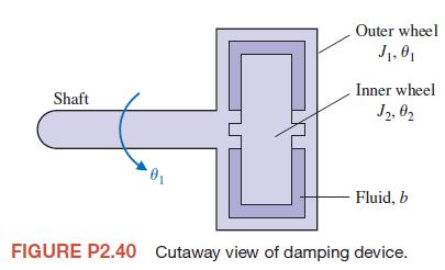
P2.40 A damping device is used to reduce the undesired vibrations of machines. A viscous fluid, such as a heavy oil, is placed between the wheels, as shown in Figure P2.40. When vibration becomes excessive, the relative motion of the two wheels creates damping.When the device is rotating without
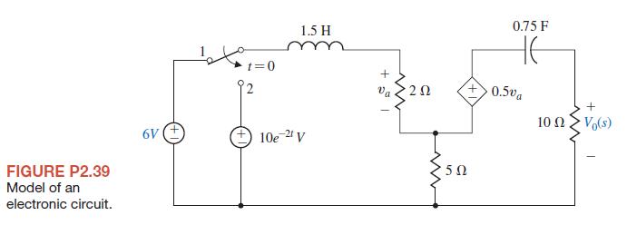
For the circuit of Figure P2.39, determine the transform of the output voltage V0 (s). Assume that the circuit is in steady state when t < 0. Assume that the switch moves instantaneously from contact 1 to contact 2 at t = 0.
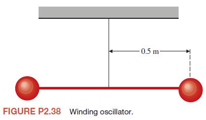
P2.38 A winding oscillator consists of two steel spheres on each end of a long slender rod, as shown in Figure P2.38. The rod is hung on a thin wire that can be twisted many revolutions without breaking. The device will be wound up 4000 degrees. How long will it take until the motion decays to a
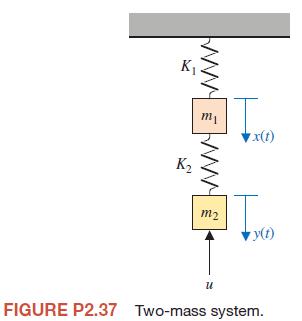
A two-mass system is shown in Figure P2.37 with an input force u(t). When m1 = m2 = 1 and K1 = K2 = 1,(a) find the set of differential equations describing the system, and (b) compute the transfer function from U(s) to Y(s). K m x(t) m2 y(t) u FIGURE P2.37 Two-mass system.
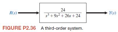
A system is represented by Figure P2.36. (a) Determine the partial fraction expansion and y(t) for a ramp input, r(t) = t, and t ≥ 0. (b) Obtain a plot of y(t)for part (a), and find y(t) for t = 1.0 s. (c) Determine the impulse response of the system y(t) for t ≥ 0. (d)Obtain a plot of y(t) for
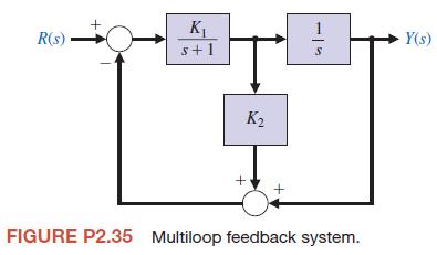
P2.35 A feedback control system has the structure shown in Figure P2.35. Determine the closed-loop transfer function Y(s)/R(s) (a) by block diagram manipulation and (b) by using a signal-flow graph and Mason’s signal-flow gain formula. (c) Select the for a unit step input. What is the time
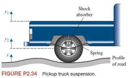
P2.34 The suspension system for one wheel of an old-fashioned pickup truck is illustrated in Figure P2.34.The mass of the vehicle is m1 and the mass of the wheel is m2. The suspension spring has a spring constant k1 and the tire has a spring constant k2. The damping constant of the shock absorber
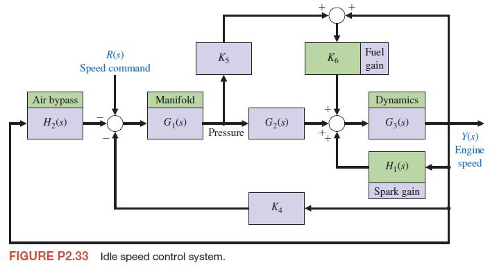
Find the transfer function for Y(s)/R(s) for the idle-speed control system for a fuel-injected engine as shown in Figure P2.33. Air bypass H(s) R(s) Speed command Manifold Fuel Ks K6 gain Dynamics G(s) G(s) G3($) Pressure Y(s) Engine FIGURE P2.33 Idle speed control system. H($) Spark gain K4 speed
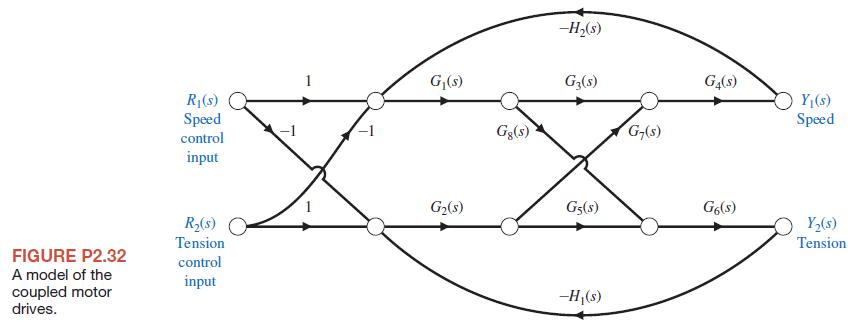
A system consists of two electric motors that are coupled by a continuous flexible belt. The belt also passes over a swinging arm that is instrumented to allow measurement of the belt speed and tension.The basic control problem is to regulate the belt speed and tension by varying the motor
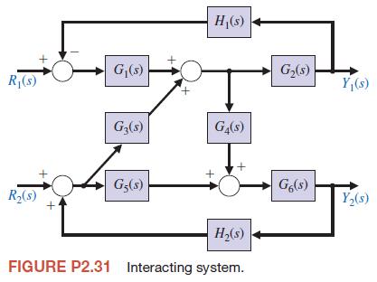
An interacting control system with two inputs and two outputs is shown in Figure P2.31. Solve for Y1 (s)/R1 (s) and Y2 (s)/R1 (s) when R2 = 0. G(s) R(s) G3($) + H(s) G4(s) + G(s) Y(s) G5(s) G6(s) R(s) + Y(s) H(s) FIGURE P2.31 Interacting system.
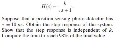
P2.30 The measurement or sensor element in a feedback system is important to the accuracy of the system [6].The dynamic response of the sensor is important.Many sensor elements possess a transfer function k H(s) = TS+1 Suppose that a position-sensing photo detector has T= 10 s. Obtain the step
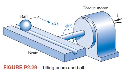
We desire to balance a rolling ball on a tilting beam as shown in Figure P2.29. We will assume the motor input current i controls the torque with negligible friction. Assume the beam may be balanced near the horizontal (φ = 0); therefore, we have a small deviation of φ(t). Find the transfer
A multiple-loop model of an urban ecological system might include the following variables: number of people in the city (P), modernization (M), migration into the city (C), sanitation facilities (S), number of diseases (D), bacteria/area (B), and amount of garbage/area (G), where the symbol for the
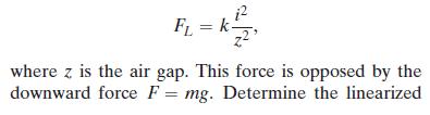
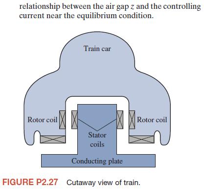
Magnetic levitation trains provide a high-speed, very low friction alternative to steel wheels on steel rails. The train floats on an air gap as shown in Figure P2.27 [25]. The levitation force FL is controlled by the coil current i in the levitation coils and may be approximated by R FL = k- where
P2.26 A robot includes significant flexibility in the arm members with a heavy load in the gripper [6, 20]. A two-mass model of the robot is shown in Figure P2.26.Find the transfer function Y(s)/ F(s). x(t) F(t) M m y(t) wwwww k FIGURE P2.26 The spring-mass-damper model of a robot arm.
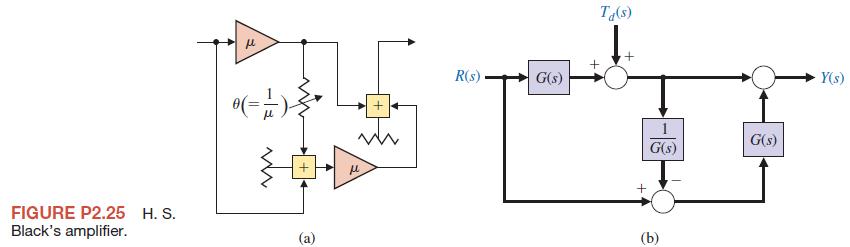
H. S. Black is noted for developing a negative feedback amplifier in 1927. Often overlooked is the fact that three years earlier he had invented a circuit design technique known as feedforward correction[19]. Recent experiments have shown that this technique offers the potential for yielding
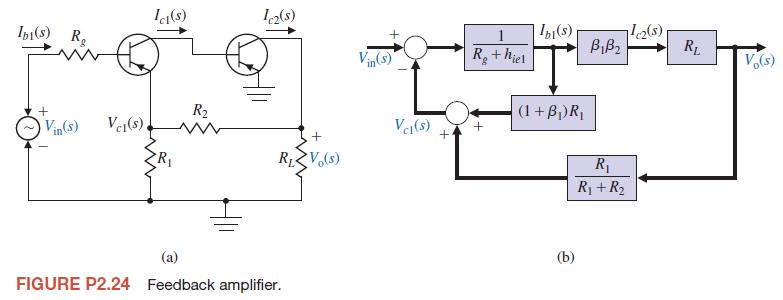
A two-transistor series voltage feedback amplifier is shown in Figure P2.24(a). This AC equivalent circuit neglects the bias resistors and the shunt capacitors.A block diagram representing the circuit is shown in Figure P2.24(b). This block diagram neglects the effect of hre, which is usually an
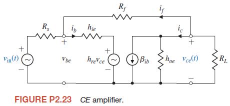
The small-signal circuit equivalent to a common-emitter transistor amplifier is shown in Figure P2.23.The transistor amplifier includes a feedback resistor Rf . Determine the input–output ratio Vce (s)/Vin (s). R if R$ in hie ww ic Vin(t) Vbe hrevce Bib hoe Vce(t) RL FIGURE P2.23 CE amplifier.
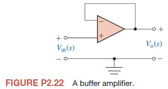
A particular form of an operational amplifier is when the feedback loop is short-circuited. This amplifier is known as a voltage follower (buffer amplifier) as shown in Figure P2.22. Show that T = Vo (s)/Vin(s) = 1.Assume an ideal op-amp. Discuss a practical use of this amplifier. Vin(s) + o +
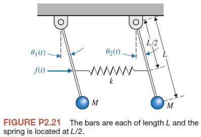
Figure P2.21 shows two pendulums suspended from frictionless pivots and connected at their midpoints by a spring [1]. Assume that each pendulum can be represented by a mass M at the end of a massless bar of length L. Also assume that the displacement is small and linear approximations can be used
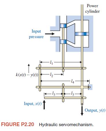
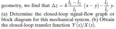
P2.20 A hydraulic servomechanism with mechanical feedback is shown in Figure P2.20 [18]. The power piston has an area equal to A. When the valve is moved a small amount Δz, the oil will flow through to the cylinder at a rate p ⋅Δz, where p is the port coefficient. The input oil pressure is
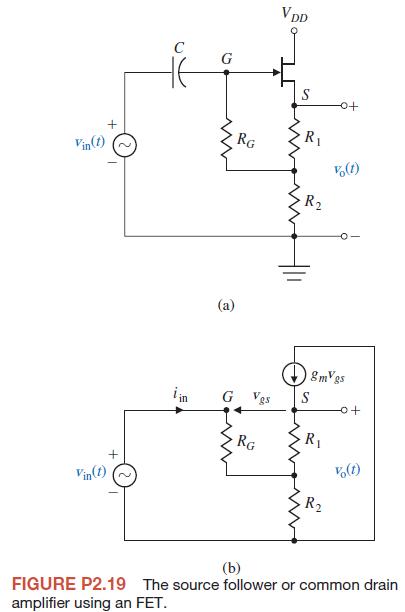
The source follower amplifier provides lower output impedance and essentially unity gain. The circuit diagram is shown in Figure P2.19(a), and the small-signal model is shown in Figure P2.19(b). This circuit uses an FET and provides a gain of approximately unity.Assume that R2 R1 for biasing
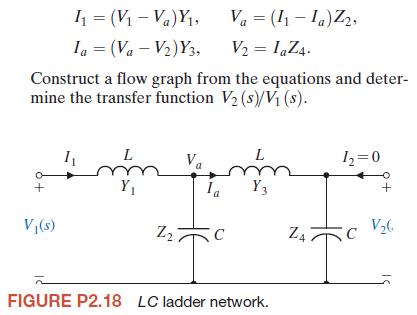
P2.18 An LC ladder network is shown in Figure P2.18.One may write the equations describing the network as follows: (V-Va), Ia = (Va - V2)Y3, Va = (1-1a)Z2, V = IaZ4. Construct a flow graph from the equations and deter- mine the transfer function V2 (s)/V (s). V(s) I Y L L 12=0 a m Ia Y3 V6 Z2 C Z4
Obtain a signal-flow graph to represent the following set of algebraic equations where x1 and x2 are to be considered the dependent variables and 6 and 11 are the inputs:Determine the value of each dependent variable by using the gain formula. After solving for x1 by Mason’s signal-flow gain
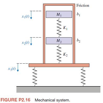
A mechanical system is shown in Figure P2.16, which is subjected to a known displacement x3 (t)with respect to the reference. (a) Determine the two independent equations of motion. (b) Obtain the equations of motion in terms of the Laplace transform, assuming that the initial conditions are
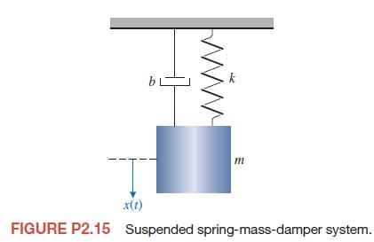
P2.15 Consider the spring-mass system depicted in Figure P2.15. Determine a differential equation to describe the motion of the mass m. Obtain the system response x(t)subjected to an impulse input with zero initial conditions. m x(t) FIGURE P2.15 Suspended spring-mass-damper system.
P2.14 A rotating load is connected to a field-controlled DC electric motor through a gear system. The motor is assumed to be linear. A test results in the output load reaching a speed of 1 rad/s within 0.5 s when a constant 80 V is applied to the motor terminals. The output steady-state speed is
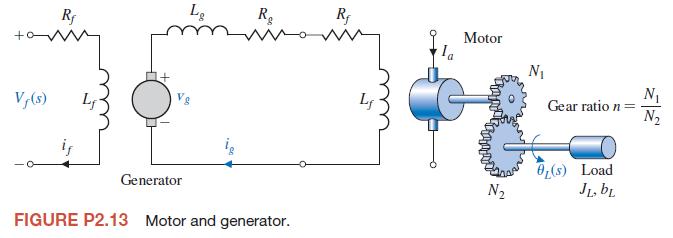
An electromechanical open-loop control system is shown in Figure P2.13. The generator, driven at a constant speed, provides the field voltage for the motor.The motor has an inertia Jm and bearing friction bm.Obtain the transfer function θL (s)/Vf (s) and draw a block diagram of the system. The
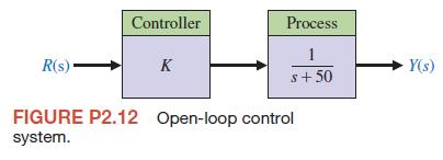
P2.12 For the open-loop control system described by the block diagram shown in Figure P2.12, determine the value of K such that y(t)→ 1 as t → ∞ when r(t) is a unit step input. Assume zero initial conditions. R(s) Controller Process 1 K Y(s) s+50 FIGURE P2.12 Open-loop control system.
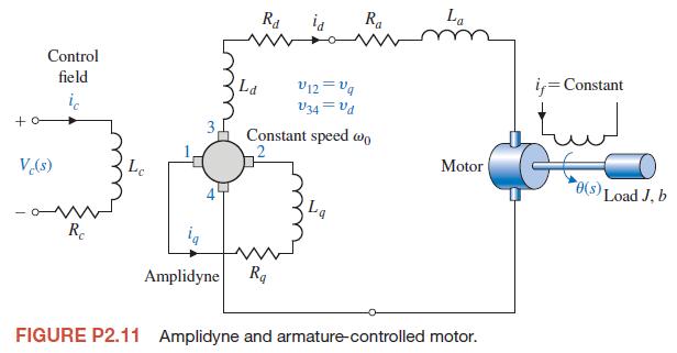
P2.11 For electromechanical systems that require large power amplification, rotary amplifiers are often used [8, 19]. An amplidyne is a power amplifying rotary amplifier.An amplidyne and a servomotor are shown in Figure P2.11. Obtain the transfer functionθ(s)/Vc (s), and draw the block diagram of
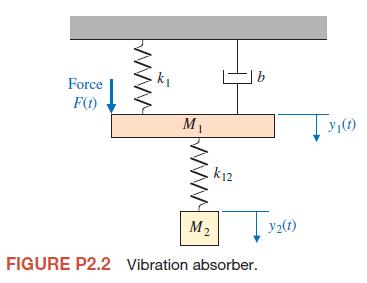
Determine the transfer function Y1 (s)/F (s) for the vibration absorber system of Problem P2.2. Determine the necessary parameters M2 and k12 so that the mass M1 does not vibrate in the steady state when F(t) = a sin(ω0t).
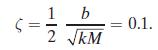
Determine the transfer function X1 (s)/F (s) for the coupled spring–mass system of Problem P2.3. Sketch the s-plane pole–zero diagram for low damping when M = 1, b/k = 1, and 1 b 2 kM = 0.1.
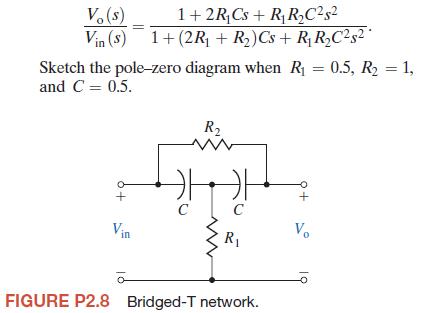
A bridged-T network is often used in AC control systems as a filter network [8]. The circuit of one bridged-T network is shown in Figure P2.8. Show that the transfer function of the network is V(s) Vin ($) 1+2RCs+ RRC 1+(2RR2)Cs + RRC* Sketch the pole-zero diagram when R = 0.5, R = 1, and C = 0.5.
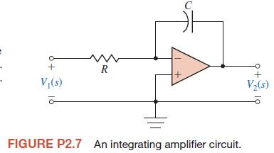
P2.7 Obtain the transfer function of the integrating amplifier circuit shown in Figure P2.7, which is an implementation of a first-order low pass filter. + V(s) www R C FIGURE P2.7 An integrating amplifier circuit. + V(s)
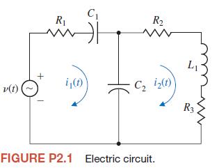
P2.6 Using the Laplace transformation, obtain the current I2 (s) of Problem P2.1. Assume that all the initial currents are zero, the initial voltage across capacitor C1 is 5υ(t), and the initial voltage across C2 is 10 volts.
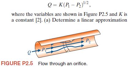
Fluid flowing through an orifice can be represented by the nonlinear equation for the fluid-flow equation. (b) What happens to the approximation obtained in part (a) if the operating point is P1 − P2 = 0? Q = K(P - P)1/2 where the variables are shown in Figure P2.5 and K is a constant [2]. (a)
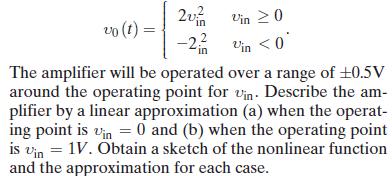
A nonlinear amplifier can be described by the following characteristic: vo (t) = -2 in vin 0 Vin
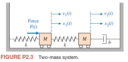
A coupled spring–mass system is shown in Figure P2.3. The masses and springs are assumed to be equal.Obtain the differential equations describing the system. V(t) V(1) Force x1(t) F(t) wwwwwM k k FIGURE P2.3 Two-mass system. N M x2(1) b
!!~!!~!!P2.2 A dynamic vibration absorber is shown in Figure P2.2. This system is representative of many situations involving the vibration of machines containing unbalanced components. The parameters M2 and k12 may be chosen so that the main mass M1 does not vibrate in the steady state when F(t) =
An electric circuit is shown in Figure P2.1. Obtain a set of simultaneous integrodifferential equations representing the network. v(t) + R www C R ww i(t) C 2(t) R3 FIGURE P2.1 Electric circuit.
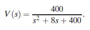
Determine the partial fraction expansion for V(s), and compute the inverse Laplace transform.The transfer function V(s) is given by V(s) = 400 + 8s + 400
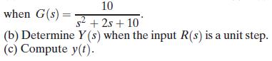
A system is shown in Figure E2.30.(a) Find the closed-loop transfer function Y(s)/R(s) 10 when G(s)= $2+2s+10 (b) Determine Y(s) when the input R(s) is a unit step. (c) Compute y(t).
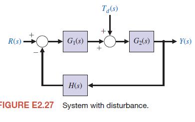
Find the transfer function Y(s)/Td (s) for the system shown in Figure E2.27. R(s) G(s) Ta(s) + G(s) Y(s) H(s) FIGURE E2.27 System with disturbance.
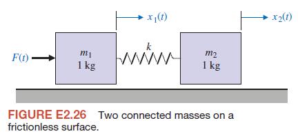
Determine the transfer function X2 (s)/F (s) for the system shown in Figure E2.26. Both masses slide on a frictionless surface and k = 1 N/m. x(t) mi F(t) www m2 1 kg 1 kg FIGURE E2.26 Two connected masses on a frictionless surface. x2(1)
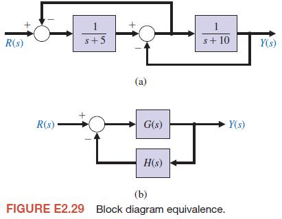
!!~!!~!!E2.29 A system is shown in Fig. E2.29(a).(a) Determine G(s) and H(s) of the block diagram shown in Figure E2.29(b) that are equivalent to those of the block diagram of Figure E2.29(a).(b) Determine Y(s)/R(s) for Figure E2.29(b). R(s) + R(s) + 1 $+5 (a) 1 s+10 Y(s) G(s) Y(s) H(s) (b) FIGURE
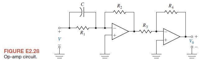
Determine the transfer function Vo(s)/V(s) for the op-amp circuit shown in Figure E2.28 [1]. Let R1 = 167 kΩ, R2 = 240 kΩ, R3 = 1 kΩ, R4 = 100 kΩ, and C = 1 μF. Assume an ideal op-amp. FIGURE E2.28 Op-amp circuit. + R R R4 R3 o+ Vo
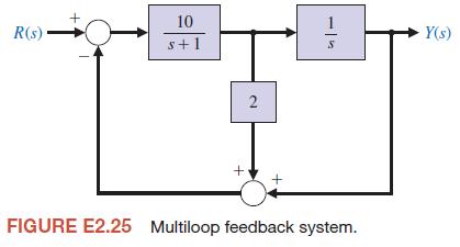
The block diagram of a system is shown in Figure E2.25. Determine the transfer function T(s) = Y(s)/R(s). R(s) + 10 s+1 2 + -5 FIGURE E2.25 Multiloop feedback system. Y(s)
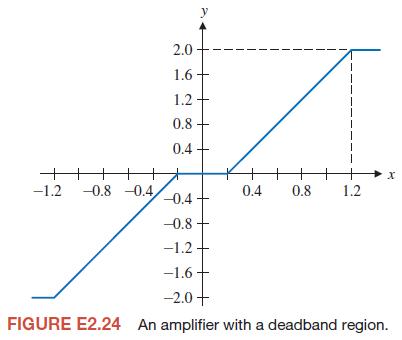
An amplifier may have a region of deadband as shown in Figure E2.24. Use an approximation that uses a cubic equation y = ax3 in the approximately linear region. Select a and determine a linear approximation for the amplifier when the operating point is x = 0.6. 2.0 1.6 1.2 0.8 0.4 y -1.2 -0.8 -0.4
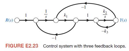
Determine the closed-loop transfer function T(s) = Y(s)/R(s) for the system of Figure E2.23. -1 S k R(s) O S Y(s) -k3 FIGURE E2.23 Control system with three feedback loops.
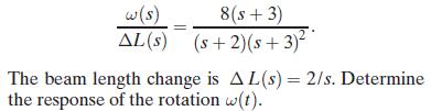
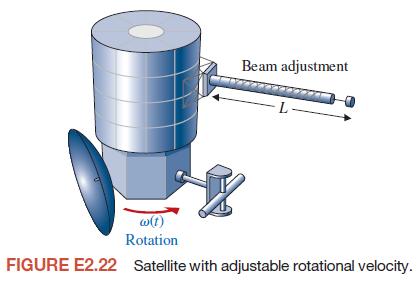
The rotational velocity ω of the satellite shown in Figure E2.22 is adjusted by changing the length of the beam L. The transfer function between ω(s) and the incremental change in beam length ΔL(s) is w(s) 8(s+3) AL(s) (s+2)(s+3)* The beam length change is AL(s) = 2/s. Determine the response of
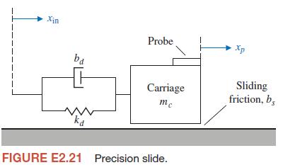
A high-precision positioning slide is shown in Figure E2.21. Determine the transfer function Xp (s)/Xin (s)when the drive shaft friction is bd = 0.7, the drive shaft spring constant is kd = 2, mc = 1, and the sliding friction is bs = 0.8. Xin bd Probe Carriage mc kd FIGURE E2.21 Precision slide. Xp
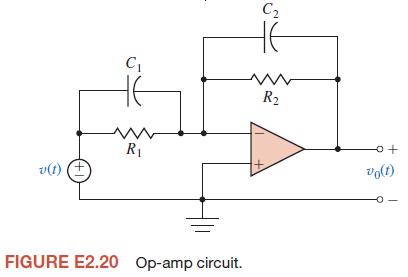
Determine the transfer function V0 (s) / V(s) of the operational amplifier circuit shown in Figure E2.20.Assume an ideal operational amplifier. Determine the transfer function when R1 = R2 = 170 kΩ, C1 =15 μF, and C2 = 25 μF. C C HE www R R v(t) 0+ + vo(t) FIGURE E2.20 Op-amp circuit.
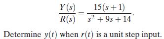
E2.19 The transfer function of a system is Y(s) 15(s+1) R(s) s+9s+14 Determine y(t) when r(t) is a unit step input.
E2.18 The output y and input x of a device are related by y = x + 1.9x3.(a) Find the values of the output for steady-state operation at the two operating points xo = 1.2 and xo = 2.5.(b) Obtain a linearized model for both operating points and compare them.
A logarithmic amplifier has a diode whose voltage is represented by the relation V = C In I, where C is a constant and I is the current across the diode. Determine a linear model for the diode when Io = 1.
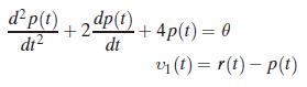
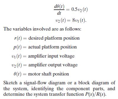
E2.16 The position control system for a spacecraft platform is governed by the following equations: dp(t) +2dp(t) 2- dt2 +4p(t) = 0 dt v(t)=r(t)-p(t)
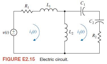
E2.15 Obtain the differential equations of the circuit in Figure E2.15 in terms of i1 (t) and i2 (t). v(t) + R L C C2. i(t) L 12(t) R FIGURE E2.15 Electric circuit.
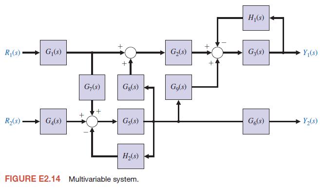
E2.14 Find the transfer functionfor the multivariable system in Figure E2.14. Y (5) R ($)
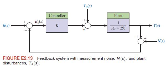
Consider the feedback system in Figure E2.13. Compute the transfer functions Y(s)/Td (s) and Y(s)/N(s) . Ta(s) Controller Plant Ea(s) + 1 R(s) K Y(s) s(s+25) FIGURE E2.13 Feedback system with measurement noise, N(s), and plant disturbances, Td(s). N(s)
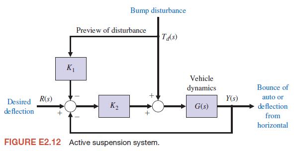
E2.12 Off-road vehicles experience many disturbance inputs as they traverse over rough roads. An active suspension system can be controlled by a sensor that looks “ahead” at the road conditions. An example of a simple suspension system that can accommodate the bumps is shown in Figure E2.12.
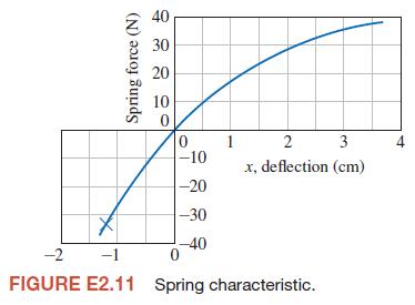
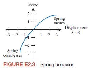
A spring exhibits a force-versus-displacement characteristic as shown in Figure E2.11. For small deviations from the operating point xo, find the spring constant when xo is (a) −1.1, (b) 0, and (c) 2.8. Spring force (N) 40 30 20 10 0 0 -10 10 -20 -30 -40 -2 -1 1 2 3 4 x, deflection (cm) FIGURE
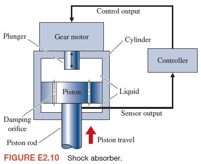
One of the beneficial applications of an automotive control system is the active control of the suspension system. One feedback control system uses a shock absorber consisting of a cylinder filled with a compressible fluid that provides both spring and damping forces [17]. The cylinder has a
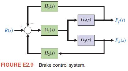
A four-wheel antilock automobile braking system uses electronic feedback to control automatically the brake force on each wheel [15]. A block diagram model of a brake control system is shown in Figure E2.9, where Ff (s) and FR(s) are the braking force of the front and rear wheels, respectively, and
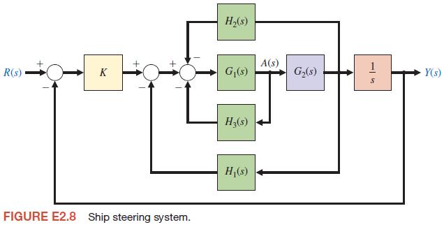
A control engineer, N. Minorsky, designed an innovative ship steering system in the 1930s for the U.S.Navy. The system is represented by the block diagram shown in Figure E2.8, where Y(s) is the ship’s course, R(s) is the desired course, and A(s) is the rudder angle [16]. Find the transfer
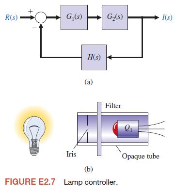
A lamp’s intensity stays constant when monitored by an optotransistor-controlled feedback loop. When the voltage drops, the lamp’s output also drops, and optotransistor Q1 draws less current. As a result, a power transistor conducts more heavily and charges a capacitor more rapidly [24]. The
A nonlinear device is represented by the function y = f (x) = Aex , where the operating point for the input x is xo = 0, where A is a constant. Determine a linear approximation valid near the operating point.
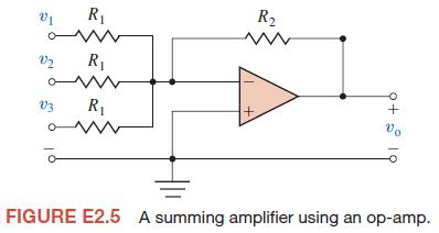
A summing amplifier uses an op-amp as shown in Figure E2.5. Assume an ideal op-amp model, and determineυo. V R R www ww D2 R 03 R www +19 FIGURE E2.5 A summing amplifier using an op-amp.
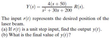
A laser printer uses a laser beam to print copy rapidly for a computer. The laser is positioned by a control input r(t), so that we have 4(s+50) Y(s) = R(s). s + 30s + 200 The input r(t) represents the desired position of the laser beam. (a) If r(t) is a unit step input, find the output y(t). (b)
The force versus displacement for a spring is shown in Figure E2.3 for the spring-mass-damper system of Figure 2.1. Graphically find the spring constant for the equilibrium point of y = 1.0 cm and a range of operation of ±2.0 cm. -3-2-1 2 1 Force Spring breaks Displacement (cm) + 1 2 3 -2 Spring
A thermistor has a response to temperature represented by o , R = R e−0.3t where Ro = 5,000 Ω, R = resistance, and T = temperature in degrees Celsius. Find the linear model for the thermistor operating at T = 20°C and for a small range of variation of temperature.
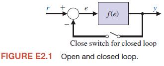
A unity, negative feedback system has a nonlinear function y = f (e) = e2, as shown in Figure E2.1. For an input r in the range of 0 to 4, calculate and plot the open-loop and closed-loop output versus input and show that the feedback system results in a more linear relationship. f(e) y Close

Showing 1000 - 1100 of 1299

1
2
3
4
5
6
7
8
9
10
11
12
13

Step by Step Answers

Services

Sitemap
Fun
Definitions
Become Tutor
Used Textbooks
Study Help Categories
Recent Questions
Expert Questions
Campus Wear
Sell Your Books

Company Info

Security
Copyrights
Privacy Policy
Terms & Conditions
SolutionInn Fee
Scholarship
Online Quiz
Give Feedback, Get Rewards

Get In Touch

About Us
Contact Us
Career
Jobs
FAQ
Student Discount
Campus Ambassador

Secure Payment

Download Our App

© 2026 SolutionInn. All Rights Reserved