New Semester
Started
Get
50% OFF
Study Help!
--h --m --s
Claim Now
Question Answers
Textbooks
Find textbooks, questions and answers
Oops, something went wrong!
Change your search query and then try again
S
Books
FREE
Study Help
Expert Questions
Accounting
General Management
Mathematics
Finance
Organizational Behaviour
Law
Physics
Operating System
Management Leadership
Sociology
Programming
Marketing
Database
Computer Network
Economics
Textbooks Solutions
Accounting
Managerial Accounting
Management Leadership
Cost Accounting
Statistics
Business Law
Corporate Finance
Finance
Economics
Auditing
Tutors
Online Tutors
Find a Tutor
Hire a Tutor
Become a Tutor
AI Tutor
AI Study Planner
NEW
Sell Books
Search
Search
Sign In
Register
study help
engineering
modern control systems
Modern Control Systems 14th Global Edition Richard Dorf, Robert Bishop - Solutions
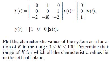
Consider the state variable model with parameter K given by x(t) = 0 1 0 0 0 1x(t)+0u(t), -2-K-2 y(t)= [100]x(t). Plot the characteristic values of the system as a func- tion of K in the range 0 < K < 100. Determine that range of K for which all the characteristic values lie in the left
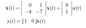
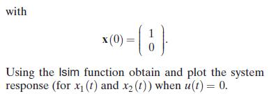
CP3.7 Consider the following system: x(t) = 0 1 x(t) -4-7 y(t)= [10]x(t)
CP3.6 Consider the closed-loop control system in Figure CP3.6.(a) Determine a state variable representation of the controller.(b) Repeat part (a) for the process.(c) With the controller and process in state variable form, use the series and feedback functions to compute a closed-loop system
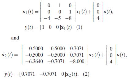
CP3.5 Consider the two systems(a) Using the tf function, determine the transfer function Y(s)/U(s) for system (1).(b) Repeat part (a) for system (2).(c) Compare the results in parts (a) and (b) and comment. and X1 (t) = 0 1 0 00 1 x1(t)+0 u(t), -4-5-8 y(t)= [100]x (t) (1) 4 0.5000 0.5000 0.7071 0
CP3.4 Consider the system(a) Using the tf function, determine the transfer function Y(s)/U(s).(b) Plot the response of the system to the initial condition x(0) = [ 0 −1 1 ]T for 0 t 20.(c) Compute the state transition matrix using the expm function, and determine x(t) at t = 20 for the initial
CP3.3 Consider the RLC circuit shown in Figure CP3.3.Determine the transfer function V2 (s)/V1(s).(a) Determine the state variable representation when R = 1 , L = 0.5 H, and C = 1 F.(b) Using the state variable representation from part (a), plot the unit step response with the step function.
By using the tf function, determine the transfer function representation for the state variable models based on your answers for CP3.1. Show that the transfer function is the same.
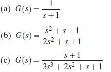
Determine a state variable representation for the following transfer functions (with unity feedback)using the ss function: (b) G(s) = (a) G(s)= 1 s+1 +s+1 2s+s+1 s+1 (c) G(s) = 353 +252 +s+1
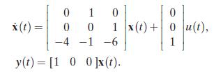
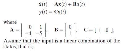
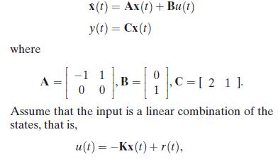
Consider the single-input, single-output system described by x(t) = Ax(t)+ Bu(t) y(t) = Cx(t) where 0 1 A B -4-5 || C=[10] Assume that the input is a linear combination of the states, that is,
DP3.4 The Mile-High Bungi Jumping Company wants you to design a bungi jumping system (that is a cord)so that the jumper cannot hit the ground when his or her mass is less than 100 kg, but greater than 50 kg. Also, the company wants a hang time (the time a jumper is moving up and down) greater than
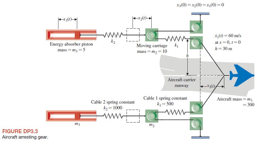
DP3.3 An aircraft arresting gear is used on an aircraft carrier as shown in Figure DP3.3. The linear model of each energy absorber has a drag force fD(t) = KDx3 (t). It is desired to halt the airplane within 30 m after engaging the arresting cable [13].The speed of the aircraft on landing is 60
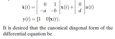
DP3.2 A system has the state variable matrix equation in phase variable formDetermine the parametersa, b, and d to yield the required diagonal matrix differential equation. x(t) = 0 1 0 (f) -a -b y(t)= [10]x(t). It is desired that the canonical diagonal form of the differential equation be
DP3.1 A spring-mass-damper system, as shown in Figure 3.3, is used as a shock absorber for a large high-performance motorcycle. The original parameters selected are m = 1 kg, b = 9 N s/m, and k = 20 N/m. (a) Determine the system matrix, the characteristic roots, and the transition matrix (t). The
The traction drive uses the capstan drive system shown in Figure CDP2.1. Neglect the effect of the motor inductance and determine a state variable model for the system. The parameters are given in Table CDP2.1. The friction of the slide is negligible.
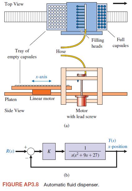
AP3.8 A system for dispensing radioactive fluid into capsules is shown in Figure AP3.8(a). The horizontal axis moving the tray of capsules is actuated by a linear motor. The x-axis control is shown in Figure AP3.8(b). (a) Obtain a state variable model of the closed-loop system with input r(t) and
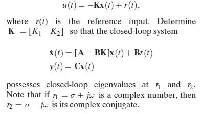
Consider the single-input, single-output system described bywhere r(t) is the reference input. The matrix K = [K1 K2 ] is known as the gain matrix. Substituting u(t) into the state variable equation gives the closed-loop system x (t) = [A −BK]x(t)+ Br(t)y(t) = Cx(t).The design process involves
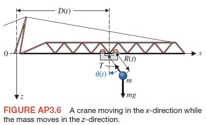
Consider a crane moving in the x direction while the mass m moves in the z direction, as shown in Figure AP3.6. The trolley motor and the hoist motor are very powerful with respect to the mass of the trolley, the hoist wire, and the load m. Consider the input control variables as the distances D(t)
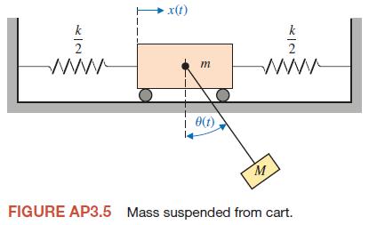
Figure AP3.5 shows a mass M suspended from another mass m by means of a light rod of length L.Obtain a state variable model using a linear model assuming a small angle for (t). Assume the output is the angle, (t). www x(t) k-2 m www i 8(t) M FIGURE AP3.5 Mass suspended from cart.
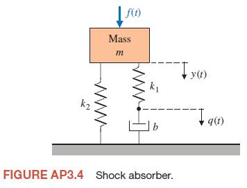
Front suspensions have become standard equipment on mountain bikes. Replacing the rigid fork that attaches the bicycle’s front tire to its frame, such suspensions absorb bump impact energy, shielding both frame and rider from jolts. Commonly used forks, however, use only one spring constant and
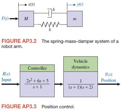
AP3.3 The control of an autonomous vehicle motion from one point to another point depends on accurate control of the position of the vehicle [16]. The control of the autonomous vehicle position Y(s) is obtained by the system shown in Figure AP3.3. Obtain a state variable representation of the
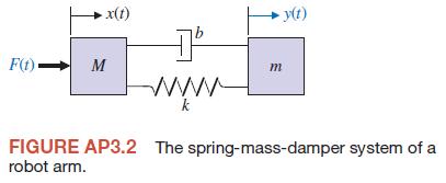
A two-mass model of a robot arm is shown in Figure AP3.2. Determine the transfer function Y(s)/F(s), and use the transfer function to obtain a state-space representation of the system. x(t) F(t) M www k m y(t) FIGURE AP3.2 The spring-mass-damper system of a robot arm.
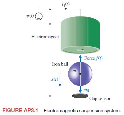
AP3.1 Consider the electromagnetic suspension system shown in Figure AP3.1. An electromagnet is located at the upper part of the experimental system. Using the electromagnetic forcef, we want to suspend the iron ball. Note that this simple electromagnetic suspension system is essentially
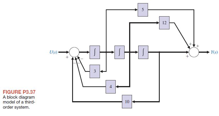
P3.37 Consider the block diagram in Figure P3.37. Using the block diagram as a guide, obtain the state variable model of the system in the form x (t) = Ax(t)+ Bu(t)y(t) = Cx(t)+ Du(t).Using the state variable model as a guide, obtain a third-order differential equation model for the system. FIGURE
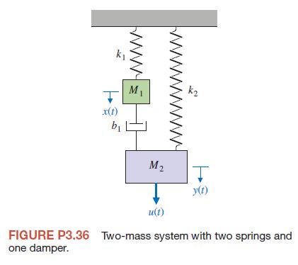
Consider the two-mass system in Figure P3.36. Find a state variable representation of the system. Assume the output is x(t). x(t) M k2 b M2 y(t) u(t) FIGURE P3.36 Two-mass system with two springs and one damper.
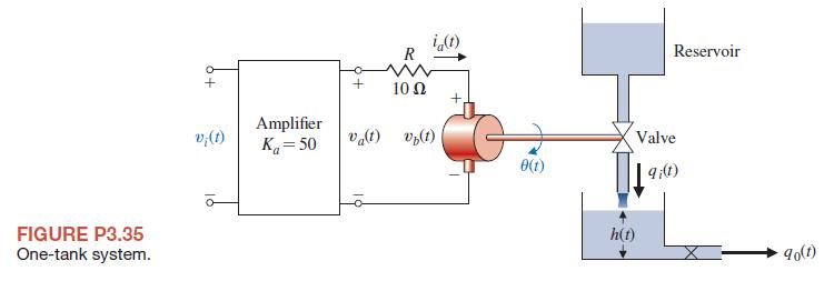
Determine a state-space representation for the system shown in Figure P3.35. The motor inductance is negligible, the motor constant is Km = 10, the back electromagnetic force constant is Kb = 0.0706, the motor friction is negligible. The motor and valve inertia is J = 0.006, and the area of the
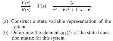
A system has the transfer function Y(s) 6 T(s)= R(s) s3+6s+11s+6 (a) Construct a state variable representation of the system. (b) Determine the element 11(t) of the state transi- tion matrix for this system.
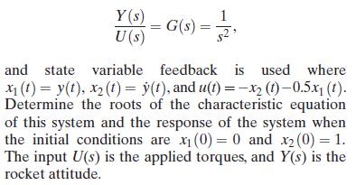
P3.33 The attitude dynamics of a rocket are represented by Y(s) G(s) = U(s) and state variable feedback is used where x1(t) = y(t), x2(t) = y(t), and u(t)=-x2 (t)-0.5x (1). Determine the roots of the characteristic equation of this system and the response of the system when the initial conditions
A drug taken orally is ingested at a rate r(t). The mass of the drug in the gastrointestinal tract is denoted by m1 (t) and in the bloodstream by m2 (t). The rate of change of the mass of the drug in the gastrointestinal tract is equal to the rate at which the drug is ingested minus the rate at
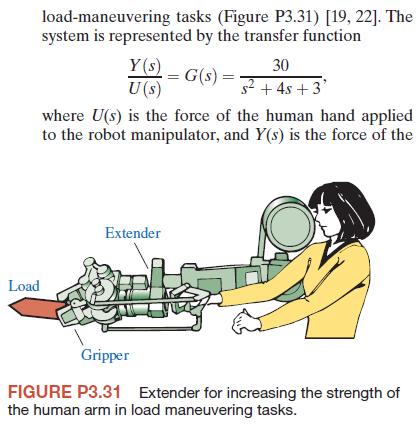
P3.31 Extenders are robot manipulators that extend(that is, increase) the strength of the human arm inrobot manipulator applied to the load. Determine a state variable model and the state transition matrix for the system. Load load-maneuvering tasks (Figure P3.31) [19, 22]. The system is
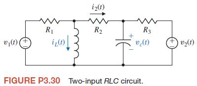
P3.30 Obtain the state equations for the two-input and one-output circuit shown in Figure P3.30, where the output is i2 (t). v(t) + i2(t) www R R R3 iz(t) v(t) FIGURE P3.30 Two-input RLC circuit. + V(1)
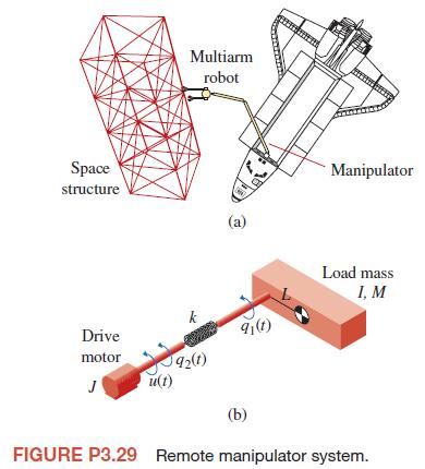
There has been considerable engineering effort directed at finding ways to perform manipulative operations in space—for example, assembling a space station and acquiring target satellites. To perform such tasks, space shuttles carry a remote manipulator system (RMS) in the cargo bay [4, 12, 21].
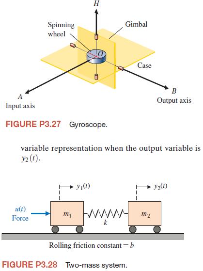
P3.28 A two-mass system is shown in Figure P3.28.The rolling friction constant isb. Determine a state Input axis Spinning wheel H Gimbal Case B Output axis FIGURE P3.27 Gyroscope. variable representation when the output variable is y2(t). y(t) u(t) Force m m2 k Rolling friction constant=b FIGURE
A gyroscope with a single degree of freedom is shown in Figure P3.27. Gyroscopes sense the angular motion of a system and are used in automatic flight control systems. The gimbal moves about the output axis OB. The input is measured around the input axis OA. The equation of motion about the output
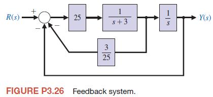
A system has a block diagram as shown in Figure P3.26. Determine a state variable model and the state transition matrix (s). R(s) 1 25 25 s+3 Y(s) S 3 25 FIGURE P3.26 Feedback system.
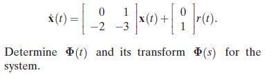
A system has the following differential equation: 0 1 x(t)= x(t) + r(t). -2-3 Determine (t) and its transform (s) for the system.
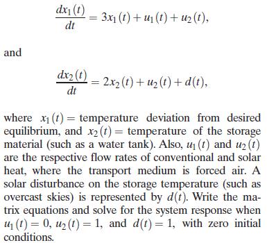
It is desirable to use well-designed controllers to maintain building temperature with solar collector space-heating systems. One solar heating system can be described by [10] and dx (t) dt 3x1 (t) + u (t) + u (t), dx2(t) = 2x2(t)+u2(t)+d(t), where x(t) dt temperature deviation from desired
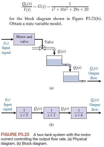
The two-tank system shown in Figure P3.23(a) is controlled by a motor adjusting the input valve and ultimately varying the output flow rate. The system has the transfer function I(s) Input signal (s) I(s) 1 == G(s) = +10s2+29s+20 for the block diagram shown in Figure P3.23(b). Obtain a state
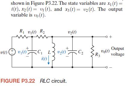
Determine a state variable model for the circuit shown in Figure P3.22. The state variables are x(t) = i(t), x2(t)= v(t), and x3 (t)=v2(t). The output variable is up (t). R v(t) R v2(t) 0+ v(t) v(1) C L V(t) "I C vo(t) Output R3 voltage i(t) FIGURE P3.22 RLC circuit.
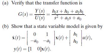
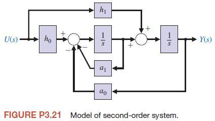
Consider the block diagram in Figure P3.21. (a) Verify that the transfer function is Y(s) hsho+ah G(s) = 2 U(s) s+as+ao (b) Show that a state variable model is given by 0 1 x(t) = -ao-a y(t)= [10]x(t). h i(t), ho
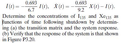
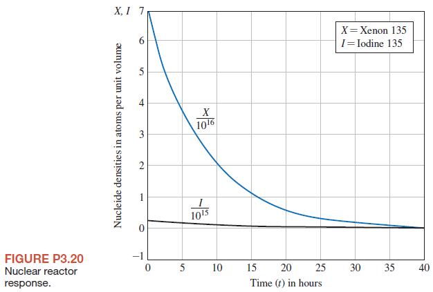
A nuclear reactor that has been operating in equilibrium at a high thermal-neutron flux level is suddenly shut down. At shutdown, the density X of xenon 135 and the density I of iodine 135 are 7×10¹⁶ and 3×10¹⁵ atoms per unit volume, respectively. The half-lives of I135 and Xe135 nucleides are
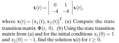
Consider the system described by 0 1 x(t)= = 4 x(t), -4-4 where x(t) = (x1(t), x2(t)). (a) Compute the state transition matrix (t, 0). (b) Using the state transition matrix from (a) and for the initial conditions x (0) = 1 and x2 (0)-1, find the solution x(t) for t 0.
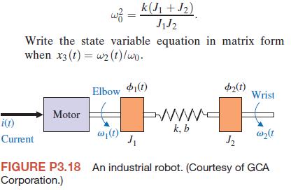
Consider the control of the robot shown in Figure P3.18. The motor turning at the elbow moves the wrist through the forearm, which has some flexibility as shown [16]. The spring has a spring constant k and friction-damping constantb. Let the state variables be x1 (t) = 1 (t)−2 (t) and x2 (t) = 1
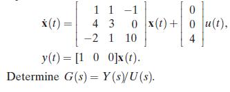
A system is described by the state variable equations 11-1 x(t) = 4 3 0 x(t)+0u(t), -21 10 y(t) = [100]x(t). Determine G(s) Y(s)/U(s). =
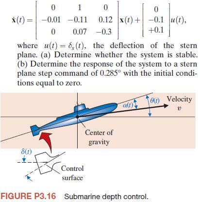
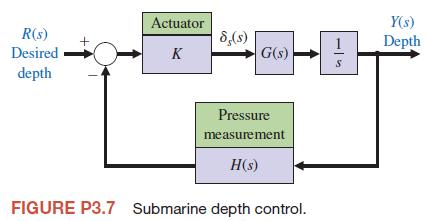
The dynamics of a controlled submarine are significantly different from those of an aircraft, missile, or surface ship. This difference results primarily from the moment in the vertical plane due to the buoyancy effect. Therefore, it is interesting to consider the control of the depth of a
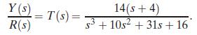
Obtain a block diagram and a state variable representation of this system. Y(s)=T(s)= R(s) 14(s+4) s3+10s2 +31s+16
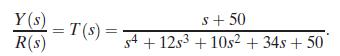
Determine a state variable representation for a system with the transfer function Y(s) R(s) s+50 =T(s)= == s4+12s3+10s2 + 34s +50
Consider again the spring-mass-damper system of Problem P3.1 when M = 1, b = 6, and k = 8. (a)Determine whether the system is stable by finding the characteristic equation with the aid of the A matrix.(b) Determine the state transition matrix of the system.(c) When the initial velocity is 1 m/s and
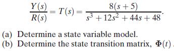
A system is described by its transfer function Y(s) 8(s+5) =T(s)= R(s) s3+12s2+44s + 48 (a) Determine a state variable model. (b) Determine the state transition matrix, (t)
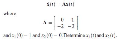
P3.11 A system is described by where x(t) = Ax(t) 0 1 A -2 -3 and x1 (0)= 1 and x2 (0) = 0. Determine x (t) and x2 (t).
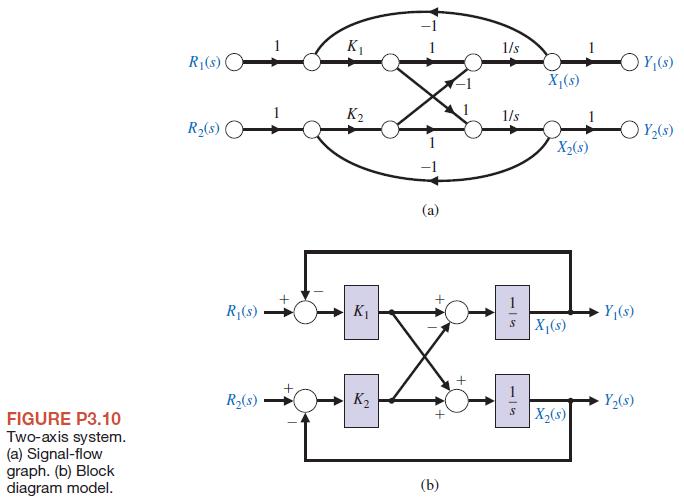
Many control systems must operate in two dimensions, for example, the x- and the y-axes. A two-axis control system is shown in Figure P3.10, where a set of state variables is identified. The gain of each axis is K1 and K2, respectively. (a) Obtain the state differential equation. (b) Find the
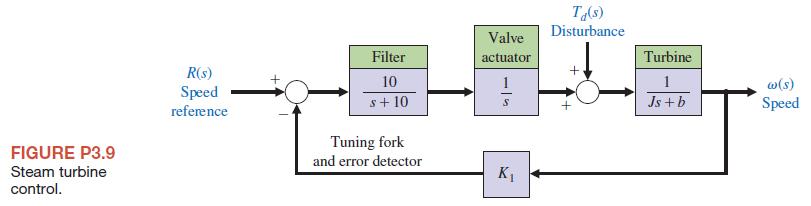
A speed control system using fluid flow components is to be designed. The system is a pure fluid control system because it does not have any moving mechanical parts. The fluid may be a gas or a liquid. A system is desired that maintains the speed within 0.5% of the desired speed by using a tuning
An automatic depth-control system for a robot submarine is shown in Figure P3.7. The depth is measured by a pressure transducer. The gain of the stern plane actuator is K = 1 when the vertical velocity is 25 m/s.The submarine has the transfer function (s+ 2) G(s) = $2+2 and the feedback transducer
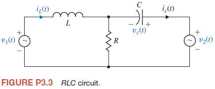
An RLC network is shown in Figure P3.3. Define the state variables as x1 (t) = iL(t) and x2 (t) = c (t).Obtain the state differential equation. v(t) iz(t) m L R FIGURE P3.3 RLC circuit. C ic(t) vc(t) + + V(1)
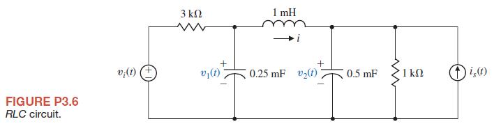
P3.6 Determine the state variable matrix equation for the circuit shown in Figure P3.6. Let x1 (t) = 1 (t), x2 (t) = 2 (t), and x3 (t) = i(t). FIGURE P3.6 RLC circuit. 3 1 mH vi(t) v(t) 0.25 mF 2(t)) 0.5 mF 1 i,(t)
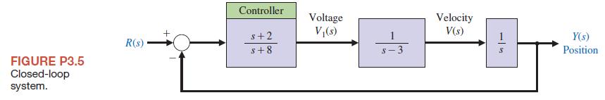
A closed-loop control system is shown in Figure P3.5. (a) Determine the closed-loop transfer function T(s) = Y(s)/R(s). (b) Determine a state variable model and sketch a block diagram model in phase variable form. 11 Controller Voltage Velocity s+2 V(s) V(s) 1 R(s) s+8 $-3 FIGURE P3.5 Closed-loop
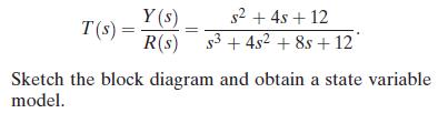
The transfer function of a system is T(s) = Y(s) s + 4s +12 = R(s) s3+4s2+8s +12 Sketch the block diagram and obtain a state variable model.
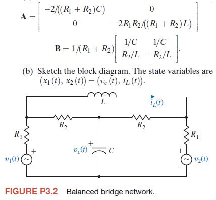
A balanced bridge network is shown in Figure P3.2.(a) Show that the A and B matrices for this circuit are -2/((R + R)C) 0 0 -2RR2/((R + R)L) 1/C 1/C B=1/(R + R) R/L -R/L (b) Sketch the block diagram. The state variables are (x1 (t), x2 (t)) = (vc (t), IL (t)). L iz(t) w R www R R R vc(t) v(t) V(1)
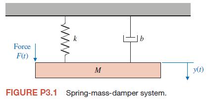
A spring-mass-damper system is shown in Figure P3.1.(a) Identify a suitable set of state variables. (b) Obtain the set of first-order differential equations in terms of the state variables. (c) Write the state differential equation. Force F(t) www M FIGURE P3.1 Spring-mass-damper system. y(t)
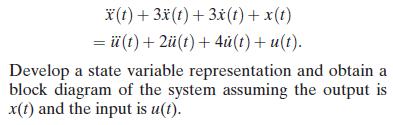
Consider a system modeled via the third-order differential equation x(t)+3x(t)+3x(t) + x(t) =(t)+2(t)+4(t) + u(t). Develop a state variable representation and obtain a block diagram of the system assuming the output is x(t) and the input is u(t).
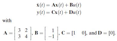
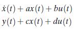
Consider the system in state variable form(a) Compute the transfer function G(s) = Y(s)/U(s).(b) Determine the poles and zeros of the system. (c) If possible, represent the system as a first-order system wherea, b,c, and d are scalars such that the transfer function is the same as obtained in (a).
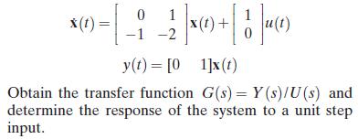
A single-input, single-output system is described by 0 x(t) = x(t) -1-2 y(t)= [01]x(t) Obtain the transfer function G(s) = Y(s)/U(s) and determine the response of the system to a unit step input.
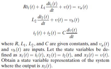
Consider a system represented by the following differential equations: Ri(t) + Ldi (t) + v(t) = va(t) dt di (t) L2 + v(t) = vp (t) dt (t) + 2(t) = cdv(t) dt where R, L1, L2, and C are given constants, and v(t) and v(t) are inputs. Let the state variables be de- fined as x(t)=(t), x2 (t)= i2(t),
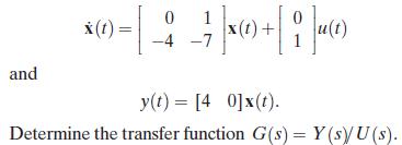
A single-input, single-output system has the matrix equations 0 x(t) = -4-7 and x(t)- u(t) y(t) = [40]x(t). Determine the transfer function G(s) = Y(s)/U(s).
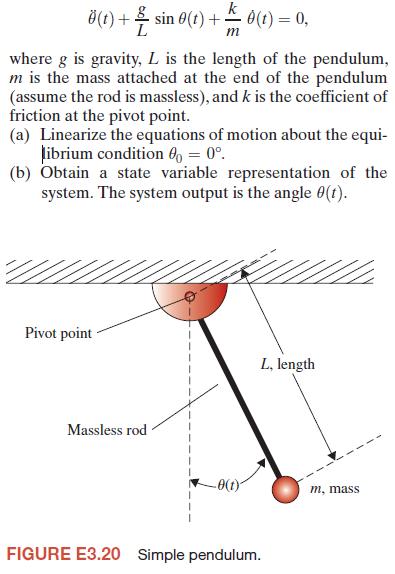
For the simple pendulum shown in Figure E3.20, the nonlinear equations of motion are given by k (t) + sin 0(t) + 0(1) = 0, L m where g is gravity, L is the length of the pendulum, m is the mass attached at the end of the pendulum (assume the rod is massless), and k is the coefficient of friction at
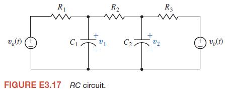
Determine a state variable differential matrix equation for the circuit shown in Figure E3.17: R R R3 www www www + va(t) + C C 1002 + v (t) V(1) FIGURE E3.17 RC circuit.
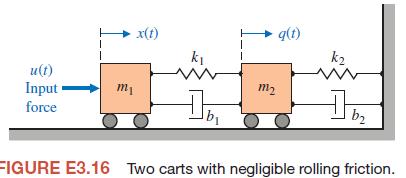
Two carts with negligible rolling friction are connected as shown in Figure E3.16. An input force is u(t).The output is the position of cart 2, that is, y(t) = q(t).Determine a state space representation of the system. u(t) Input force x(t) (1)b+ k k2 www m m2 b b FIGURE E3.16 Two carts with
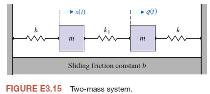
E3.15 Consider the case of the two masses connected as shown in Figure E3.15. The sliding friction of each mass has the constantb. Determine a state variable matrix differential equation. x(t) kj m q(t) m W Sliding friction constant b FIGURE E3.15 Two-mass system.
Develop the state-space representation of a radioactive material of mass M to which additional radioactive material is added at the rate r(t) = Ku(t), where K is a constant. Identify the state variables. Assume that the mass decay is proportional to the mass present.
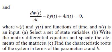
A system is described by the two differential equations dy(t) + y(t)-2u(t) + aw(t) = 0, dt
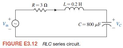
Use a state variable model to describe the circuit of Figure E3.12. Obtain the response to an input unit step when the initial current is zero, and the initial capacitor voltage is zero. Vin R=3 L= 0.2 H C=800 F + FIGURE E3.12 RLC series circuit. Vc
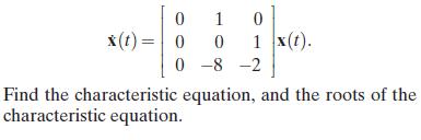
Consider the system 0 1 0 x(t)=0 0 1 x(t). 0-8-2 Find the characteristic equation, and the roots of the characteristic equation.
Consider the spring and mass shown in Figure 3.3 where M = 1 kg, k = 100 N/m, and b = 20 Ns/m.(a) Find the state vector differential equation. (b) Find the roots of the characteristic equation for this system.
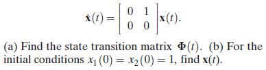
Consider the system 0 x(t)= x(t). 0 (a) Find the state transition matrix initial conditions x (0) = x2 (0) = 1, find x(t). (t). (b) For the
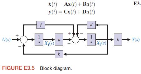
A system is represented by a block diagram as shown in Figure E3.5. Write the state equations in the form f x(t) Ax(t)+ Bu(t) y(t)=Cx(t)+ Du(t) d E3. U(s) a S X(s) k FIGURE E3.5 Block diagram. + b Y(s) X2(s)
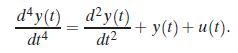
Obtain a state variable matrix for a system with a differential equation dy(t) dy(t) + y(t)+u(t). dt4 dt
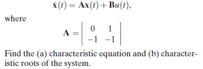
The system in E3.3 can be represented by the state vector differential equation x(t) Ax(t)+ Bu(t), where 0 1 A -1 - Find the (a) characteristic equation and (b) character- istic roots of the system.
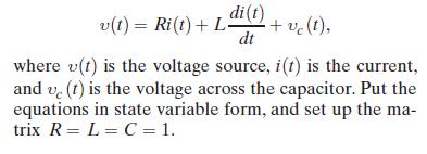
The voltage-current relationship for a series RLC circuit can be represented by the differential equation v(t) = Ri(t) + Li(t) +ve (1), dt where v(t) is the voltage source, i(t) is the current, and ve (t) is the voltage across the capacitor. Put the equations in state variable form, and set up the
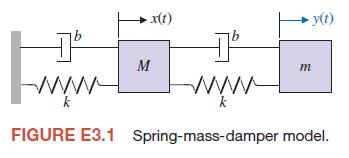
For the spring-mass-damper model shown in Figure E3.1, identify a set of state variables. www M k x(t) www k m y(t) FIGURE E3.1 Spring-mass-damper model.
A system is represented by the transfer function Y(s) R(s) 5(s+10) T(s) = s3+10s2+20s +50
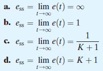
The steady-state error E(s) = Y(s)− R(s) due to a unit step disturbance Td (s) = 1 / s is: a. ess = lim e(t) = xx 1-00 b. ess = lim e(t)=1 1-00 1 c. ess = lim e(t)= = 1- K+1 d. ess = lim e(t) = K +1 0041
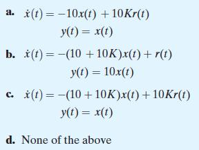
13. The state-space representation of the closed-loop system from R(s) to Y(s) is: a. x(t)=-10x(t) + 10Kr(t) y(t) = x(t) b. x(t)=(10+10K)x(t) + r(t) y(t) = 10x(t) c. x(t)=(10+10K)x(t) + 10Kr(t) y(t) = x(t) d. None of the above
The effect of the input R(s) and the disturbance Td (s) on the output Y(s) can be considered independently of each other because:a. This is a linear system, therefore we can apply the principle of superposition.b. The input R(s) does not influence the disturbance Td (s).c. The disturbance Td (s)
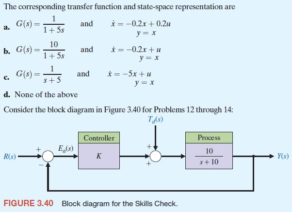
A first-order dynamic system is represented by the differential equation 5x(t)+ x(t) = u(t). The corresponding transfer function and state-space representation are a. G(s) = 1 1+5s and x = -0.2x + 0.2u y = x 10 b. G(s) = and x=-0.2x+u 1+5s y = x 1 C. G(s) = and x = -5x+u $ +5 y = x d. None of the
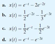
The differential equation model for two first-order systems in series is x(t)+ 4x(t)+ 3x(t) = u(t), where u(t) is the input of the first system and x(t) is the output of the second system. The response x(t) of the system to a unit impulse u(t) is: a. x(t)=e-2e-21 1 b. x(t)= -21 = - 1 -31 -e 3 CG
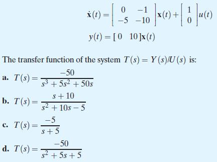
A single-input, single-output system has the state variable representation 0-1 x(t) = |x(t) + -5-10 y(t) [010]x(t) The transfer function of the system T(s) = Y(s)/U(s) is: a. T(s)= -50 $3+5s2 +50s s+10 b. T(s)= $+10s-5 -5 c. T(s)= $+5 -50 d. T(s)=2+5s+5
For the initial conditions x1 (0) = x2 (0) = 1, the response x(t) for the zero-input response is:a. x1 (t) = (1 + t), x2 (t) = 1 for t 0b. x1 (t) = (5 + t), x2 (t) = t for t 0c. x1 (t) = (5t + 1), x2 (t) = 1 for t 0d. x1 (t) = x2 (t) = 1 for t 0
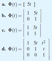
The associated state-transition matrix is: a. (t)= [51] 1 5t b. (t) 01 1 5t c. (t)= = 1 1 5t t d. (t)=0 1 t 001
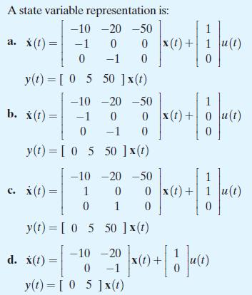
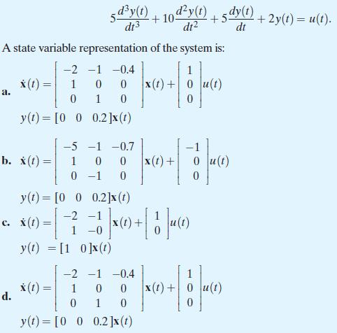
Consider a system with the mathematical model given by the differential equation: 5dy(t) dt3 +10 dy (1) dt +5dy(1) dt +2y(t) = u(t). A state variable representation of the system is: -2 -1 -0.4 x(t) = 1 0 0 x(t) + u(t) a. 0 1 0 y(t)= [0_0_0.2]x(t) -5 -1 -0.7 b. x(t)= 1 0 0 x(t)+ 0 u(t) y(t) c.
5. A state variable representation of a system can always be written in diagonal form. True or False
4. A time-invariant control system is a system for which one or more of the parameters of the system may vary as a function of time. True or False
3. The outputs of a linear system can be related to the state variables and the input signals by the state differential equation. True or False
2. The matrix exponential function describes the unforced response of the system and is called the state transition matrix. True or False
1. The state variables of a system comprise a set of variables that describe the future response of the system, when given the present state, all future excitation inputs, and the mathematical model describing the dynamics. True or False
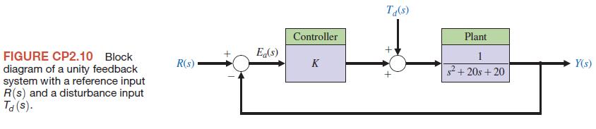
Consider the block diagram in Figure CP2.10.Create an m-file to complete the following tasks:(a) Compute the step response of the closed-loop system (that is, R(s) = 1/s and Td (s) = 0) and plot the steady-state value of the output Y(s) as a function of the controller gain 0 (b) Compute the
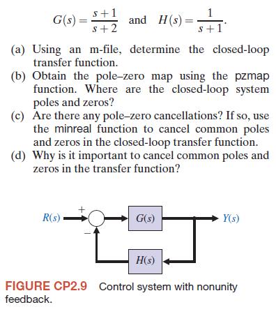
Consider the feedback control system in Figure CP2.9, where s+1 G(s) = = 5+2 and H(s)= 1 s+1 (a) Using an m-file, determine the closed-loop transfer function. (b) Obtain the pole-zero map using the pzmap function. Where are the closed-loop system poles and zeros? (c) Are there any pole-zero
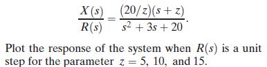
A system has a transfer function X(s) (20/z)(s+ z) R(s) s+3s+20 Plot the response of the system when R(s) is a unit step for the parameter z = 5, 10, and 15.
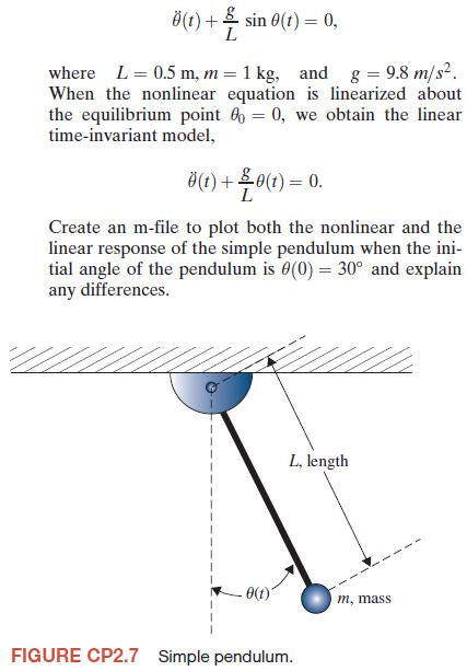
CP2.7 For the simple pendulum shown in Figure CP2.7, the nonlinear equation of motion is given by (1) +15 sin (t) = 0, where L = 0.5 m, m = 1 kg, and g = 9.8 m/s. When the nonlinear equation is linearized about the equilibrium point = 0, we obtain the linear time-invariant model, (1) +0(1) = 0. L
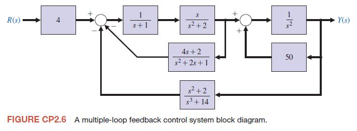
Consider the block diagram in Figure CP2.6.(a) Use an m-file to reduce the block diagram in Figure CP2.6, and compute the closed-loop transfer function.(b) Generate a pole–zero map of the closed-loop transfer function in graphical form using the pzmap function.(c) Determine explicitly the poles
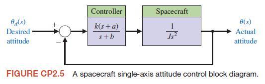
A satellite single-axis attitude control system can be represented by the block diagram in Figure CP2.5.The variables k,a, and b are controller parameters,and J is the spacecraft moment of inertia. Suppose the nominal moment of inertia is J = 10.8E8(slug ft2 ), and the controller parameters are k =
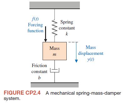
Consider the mechanical system depicted in Figure CP2.4. The input is given by f (t), and the output is y(t). Determine the transfer function from f (t)to y(t) and, using an m-file, plot the system response to a unit step input. Let m = 10, k = 1, and b = 0.5.Show that the peak amplitude of the
Showing 900 - 1000
of 1299
1
2
3
4
5
6
7
8
9
10
11
12
13
Step by Step Answers