New Semester Started Get 50% OFF Study Help! --h --m --s Claim Now

Question Answers

Textbooks

Find textbooks, questions and answers

Oops, something went wrong!

Change your search query and then try again

Result Not Found

Books FREE
Study Help
Tutors
AI Study Planner NEW
Sell Books

Search
Sign In
Register

study help
business
probability and stochastic modeling

An Introduction To Stochastic Modeling 3rd Edition Samuel Karlin, Howard M. Taylor - Solutions

5.2. Let _S(t) be the position process corresponding to an Ornstein-Uhlenbeck velocity V(t). Assume that S(0) = V(0) = 0. Obtain the covariance between S(t) and V(t).
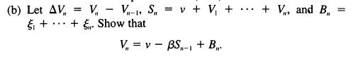
5.1. Let e,, e,, ... be independent standard normal random variables and /3 a constant, 0 Uhlenbeck process may be constructed by setting(a) Show thatComment on the comparison with (5.22).Compare and contrast with (5.24). Vov and V = (1B)V + for n1.
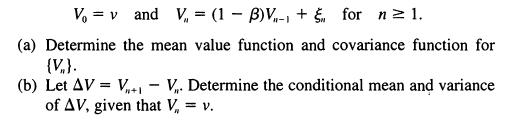
5.3. Let ,, 62, ... be independent standard normal random variables and /3 a constant, 0 Uhlenbeck process may be constructed by setting V = v and V = (1 - )V + for n 1. (a) Determine the mean value function and covariance function for (V.). - (b) Let AV = V+ V. Determine the conditional mean and
5.2. The velocity of a certain particle follows an Ornstein-Uhlenbeck process with .2 = 1 and /3 = 0.2. The particle starts at rest (v = 0) from position S(0) = 0. What is the probability that it is more than one unit away from its origin at time t = 1. What is the probability at times t = 10 and t
5.1. An Ornstein-Uhlenbeck process V(t) has 0-2 = 1 and /3 = 0.2. What is the probability that V(t)
4.10. Let to = 0 where Z(t) is geometric Brownian motion with drift parametersr and variance parameter 022 (see the geometric Brownian motion in the Black-Scholes formula (4.20)). Show that is a martingale. exp(-rt),
4.9. Let r be the first time that a standard Brownian motion B(t) starting from B(0) = x > 0 reaches zero. Let A be a positive constant. Show that w(x) = E[e-ATIB(0) = x] = e-'-21*.Hint: Develop an appropriate differential equation by instituting an infinitesimal first step analysis according to
4.8. Verify the Hewlett-Packard option valuation of $6.03 stated in the text when T = ;, z = $59, a = 60, r = 0.05 anda- = 0.35. What is the Black-Scholes valuation if o- = 0.30?
4.7. A call option is said to be "in the money" if the market price of the stock is higher than the striking price. Suppose that the stock follows a geometric Brownian motion with drifta, variance a2 , and has a current market price of z. What is the probability that the option is in the money at
4.6. What is the probability that a geometric Brownian motion with drift parameter a = 0 ever rises to more than twice its initial value? (You buy stock whose fluctuations are described by a geometric Brownian motion with a = 0. What are your chances to double your money?)
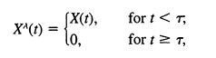
4.5. Change a Brownian motion with drift X(t) into an absorbed Brownian motion with drift X(t) by definingwhere T = min{t ? 0; X(t) = 0).(We suppose that X(0) = x > 0 and that A x? (x(t), X^(t) = 10. for t
4.4. A Brownian motion X(t) either (i) has drift μ = μ0i or (ii) has driftμ = μ,, where μ.° < μ, are known constants. It is desired to determine which is the case by observing the process. Derive a sequential decision procedure that meets prespecified error probabilities a and 0. Hint: Base
4.3. If B°(s), 0 is a standard Brownian motion. Use this representation and the result of Problem 4.2 to show that for a Brownian bridge B°(t), B(1) = (1 + 1)B( 1 + 1) t +1
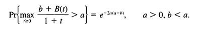
4.2. Show that Pr max 120 b+ B(t) 1+t 2 > a} = e=data-m -Za(a-b) a > 0, b
4.1. What is the probability that a standard Brownian motion {B(t) }ever crosses the line a + bt (a > 0, b > 0)?
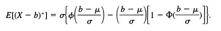
4.6. Let be a standard normal random variable.(a) For an arbitrary constanta, show that E[(e - a)+] = 4(a) - a[1 - 4)(a)](b) Let X be normally distributed with mean μ and variance cr2. Show that E[(x - b) - [6 ()- ( - ) [ - * )]} =
4.5. Suppose that the fluctuations in the price of a share of stock in a certain company are well described by a geometric Brownian motion with drift a = -0.1 and variance cr-2 = 4. A speculator buys a share of this stock at a price of $100 and will sell if ever the price rises to $110 (a profit)
4.4. A Brownian motion X(t) either (i) has drift p. = +16 > 0, or (ii) has drift μ = -ZS < 0, and it is desired to determine which is the case by observing the process for a fixed duration T. If X(T) > 0, then the decision will be that μ = +ZS; If X(T) :5 0, then μ = -ZS will be stated. What
4.3. A Brownian motion {X(t)} has parameters μ = 0.1 and a = 2.Evaluate the mean time to exit the interval (a, b] from X(0) = 0 for b =1, 10, and 100 and a = -b. Can you guess how this mean time varies with b for b large?
4.2. A Brownian motion {X(t)} has parameters μ = 0.1 anda- = 2.Evaluate the probability of exiting the interval (a, b] at the point b starting from X(0) = 0 for b = 1, 10, and 100 and a = -b. Why do the probabilities change when alb is the same in all cases?
4.1. A Brownian motion {X(t)} has parameters μ = -0.1 anda- = 2.What is the probability that the process is above y = 9 at time t = 4, given that it starts at x = 2.82?
3.9. Let F(t) be a cumulative distribution function and B°(u) a Brownian bridge.(a) Determine the covariance function for B°(F(t)).(b) Use the central limit principle for random functions to argue that the empirical distribution functions for random variables obeying F(t) might be approximated by
3.8. Show that the transition densities for both reflected Brownian motion and absorbed Brownian motion satisfy the diffusion equation (1.3) in the region 0 < x < oo.
3.7. Let to = 0 < t, < t2 < ... be time points, and define X,, = A(t,,), where A(t) is absorbed Brownian motion starting from A(0) = x. Show that is a nonnegative martingale. Compare the maximal inequality(5.7) in II with the result in Problem 3.6.
3.6. Let M = max{A(t); t 0} be the largest value assumed by an absorbed Brownian motion A(t). Show that Pr{M > zIA(0) = x} = x/z for 0
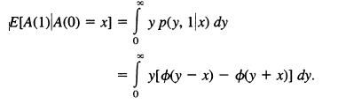
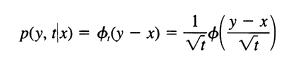
3.5. Determine the expected value for absorbed Brownian motion A(t)at time t = 1 by integrating the transition density (3.6) according toThe answer is E[A(1)IA(0) = x] = x. Show that E[A(t)IA(0) = x] = x for all t > 0. E[A(1) A(0) = x] = y p(y, 1x) dy = { = 0 - - y[oy x) (y + x)] dy.
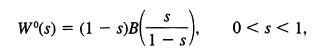
3.4. Let B(t) be a standard Brownian motion. Determine the covariance function forand compare it to that for a Brownian bridge. - W(s) = (1 s)B(1 - s. 0 < s
3.3. Let B(t) be a standard Brownian motion. Show that B(u) - uB(1), 0 < u < 1, is independent of B(1).(a) Use this to show that B°(t) = B(t) - tB(1), 0 s t < 1, is a Brownian bridge.(b) Use the representation in (a) to evaluate the covariance function for a Brownian bridge.
3.2. Let B(t) be a standard Brownian motion process. Determine the conditional mean and variance of B(t), 0 < t < 1, given that B(1) = b.
3.1. Let B,(t) and B,(t) be independent standard Brownian motion processes. DefineR(t) is the radial distance to the origin in a two-dimensional Brownian motion.Determine the mean of R(t). R(t) = B(t) + B(t), 10.
3.5. Is reflected Brownian motion a Gaussian process? Is absorbed Brownian motion (cf. Section 1.4)?
3.4. Suppose that the net inflows to a reservoir follow a Brownian motion.Suppose that the reservoir was known to be empty 25 time units ago but has never been empty since. Use a Brownian meander process to evaluate the probability that there is more than 10 units of water in the reservoir today.
3.3. The net inflow to a reservoir is well described by a Brownian motion.Because a reservoir cannot contain a negative amount of water, we suppose that the water level R(t) at time t is a reflected Brownian motion.What is the probability that the reservoir contains more than 10 units of water at
3.2. The price fluctuations of a share of stock of a certain company are well described by a Brownian motion process. Suppose that the company is bankrupt if ever the share price drops to zero. If the starting share price is A(0) = 5, what is the probability that the company is bankrupt at time t =
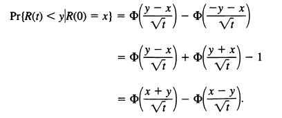
3.1. Show that the cumulative distribution function for reflected Brownian motion isEvaluate this probability when x = 1, y = 3, and t = 4. Pr(R(t) < y)R(0) = x) = 0 (2*) (-1-*) y x =(2-3)+(3+*)-1 +y' = (x+7) - (*-7).
2.6. Use the result of Problem 2.5 to show that Y(t) = M(t) - B(t) has the same distribution as JB(t)I.
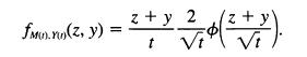
2.5. Show that the joint density function for M(t) and Y(t) = M(t) - B(t)is given by fmun.run(z, y) z+y 2 (z+y\ = t Vi Vil
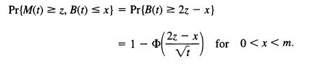
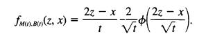
2.4. Use the reflection principle to obtain(M(t) is the maximum defined in (2.1).) Differentiate with respect to x, and then with respect to z, to obtain the joint density function for M(t) and B(t): Pr{M(t)z, B(t) x} = Pr{B(t) = 2z - x} = 1- (22-8) for 0
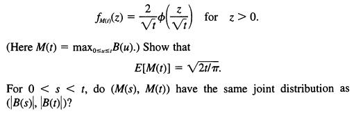
2.3. For a fixed t > 0, show that M(t) and I B(t)I have the same marginal probability distribution, whence Fan(2) = 2,0 (77) for z> 0. (Here M(t) =max,B(u).) Show that E[M(t)] = 21/TT. == For 0
2.2. Find the conditional probabiiity that a standard Brownian motion is not zero in the interval (0, b] given that it is not zero in the interval (0, a], where 0 < a
2.1. Find the conditional probability that a standard Brownian motion is not zero in the interval (t, t + b] given that it is not zero in the interval(t, t + a], where 0 < a < b and t > 0.
2.6. Let T, be the smallest zero of a standard Brownian motion that exceeds b > 0. Show that 2 Pr{T,
2.5. Let ro be the largest zero of a standard Brownian motion not exceeding a > 0. That is, To = max {u ? 0; B(u) = 0 and u < a}. Show that
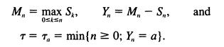
2.4. Consider the simple random walkin which the summands are independent with Pr{ = ±1) = z. Let Mn = maxo S = 0,
2.3. Suppose that net inflows to a reservoir are described by a standard Brownian motion. If at time 0 the reservoir has x = 3.29 units of water on hand, what is the probability that the reservoir never becomes empty in the first t = 4 units of time?
2.2. Show that arctanst = arccos/t/(s + t).
2.1. Let {B(t); t ? 0} be a standard Brownian motion, with B(0) = 0, and let M(t) = max{B(u); 0 s u < t}.(a) Evaluate Pr(M(4) c} = 0.10.
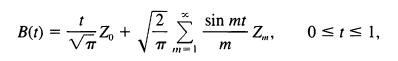
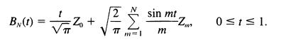
1.8. Computer Challenge A problem of considerable contemporary importance is how to simulate a Brownian motion stochastic process. The invariance principal provides one possible approach. An infinite series expression that N. Wiener introduced may provide another approach. Let Z,,, Z,, ... be a
1.7. For n = 0, 1, ... , show that (a) B(n) and (b) B(n)2 - n are martingales(see II, Section 5).
1.6. Manufacturers of crunchy munchies such as cheese crisps use compression testing machines to gauge product quality. The crisp, or whatever, is placed between opposing plates, which then move together.As the crisp is crunched, the force is measured as a function of the distance that the plates
1.5. Consider the simple random walkin which the summands are independent with Pr{ 11 _ 2W e are going to stop this random walk when it first drops a units below its maximum to date. Accordingly, let(a) Use a first step analysis to show that(b) Why is Pr{M, 2} = Pr{M, ? 1 }2, andIdentify the
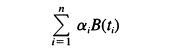
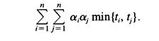
1.4. Let a,, ... , a,, be real constants. Argue thatis normally distributed with mean zero and variance a,B(t) =1
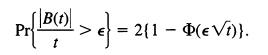
1.3. For a positive constante, show thatHow does this behave when t is large (t - x)? How does it behave when t is small (t - 0)? Pr{\B(1)\ > e} = = 2{1-(et)}.
1.2. Evaluate E[eA°"'] for an arbitrary constant A and standard Brownian motion B(t).
1.1. Consider the simple random walkin which the summands are independent with Pr{ = ± 1 } = 2I n III, Section 5.3, we showed that the mean time for the random walk to first reach -a 0 is ab. Use this together with the invariance principle to show that E[T] = ab, where T = Ta.h = min(t ? 0; B(t)
1.7. Suppose that in the absence of intervention, the cash on hand for a certain corporation fluctuates according to a standard Brownian motion{B(t); t ? 0 }. The company manages its cash using an (s, S) policy: If the cash level ever drops to zero, it is instantaneously replenished up to level s;
1.6. Consider a standard Brownian motion {B(t); t ? 0} at times 0 < u < u + v < u + v + w, where u, v, w > 0.(a) What is the probability distribution of B(u) + B(u + v)?(b) What is the probability distribution of B(u) + B(u + v) +B(u + v + w)?
1.5. Determine the covariance functions for the stochastic processes(a) U(t) = e-'B(e2i), for t:::, 0.(b) V(t) = (1 - t)B(tl(1 - t)), for 0 < t < 1.(c) W(t) = tB(1/t), with W(0) = 0.B(t) is standard Brownian motion.
1.4. Consider a standard Brownian motion {B(t); t >_ 0) at times 0 < u < u + v < u + v + w, where u, v, w > 0.(a) Evaluate the product moment E[B(u)B(u + v)B(u + v + w)].(b) Evaluate the product moment E[B(u)B(u + v)B(u + v + w)B(u + v + w + x)]where x > 0.
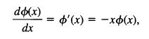
1.3.(a) Show thatwhere ¢(x) is given in (1.5).(b) Use the result in (a) together with the chain rule of differentiation to show thatsatisfies the diffusion equation (1.3). do(x) '(x) = -x+(x), dx
1.2. Let {B(t); t j 0) be a standard Brownian motion and c > 0 a constant.Show that the process defined by W(t) = cB(tlc2) is a standard Brownian motion.
1.1. Let (B(t); t ? 0) be a standard Brownian motion.(a) Evaluate Pr{B(4) : 3IB(0) = 1).(b) Find the number c for which Pr(B(9) > cl B(0) = 1) = 0.10.
6.4. Determine the long run population growth rate for a population whose individual net maternity function is mo = m, = 0 and m2 =m, = = a > 0. Compare this with the population growth rate when m,=a, andm,=0fork 2.
6.3. Determine the long run population growth rate for a population whose individual net maternity function is m, = m; = 2, and mk = 0 otherwise. Why does delaying the age at which offspring are first produced cause a reduction in the population growth rate? (The population growth rate when m, = m,
6.2. Marlene has a fair die with the usual six sides. She throws the die and records the number. She throws the die again and adds the second number to the first. She repeats this until the cumulative sum of all the tosses first exceeds a prescribed number n. (a) When n = 10, what is the
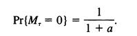
6.1. Suppose the lifetimes X, X2, ... have the geometric distribution Pr{X1 = k} = a(l - a)k-' fork = 1, 2, ... , where 0
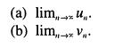
6.3. Using the data of Exercises 6.1 and 6.2, determine (a) limu. (b) lim,, V.
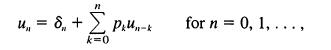
6.2. (Continuation of Exercise 6.1)(a) Solve for u,, for n = 0, 1, ... , 10 in the renewal equationwhere So = 1, S, = S, _ = 0, and {pk} is as defined in Exercise 6.1.(b) Verify that the solution v,, in Exercise 6.1 and u,, are related according to u = 8 + k=0 Pkun-k for n = 0, 1, ...,
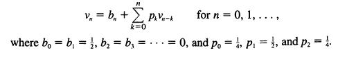
6.1. Solve for v,, for n = 0, 1, ... , 10 in the renewal equation = v = b + n k=0 where bob, , b = b = PkVa-k for n 0, 1, ..., = 0, and po = , p = 1, and p =
5.4. A lazy professor has a ceiling fixture in his office that contains two light bulbs. To replace a bulb, the professor must fetch a ladder, and being lazy, when a single bulb fails, he waits until the second bulb fails before replacing them both. Assume that the length of life of the bulbs are
5.3. At the beginning of each period, customers arrive at a taxi stand at times of a renewal process with distribution law F(x). Assume an unlimited supply of cabs, such as might occur at an airport. Suppose that each customer pays a random fee at the stand following the distribution law G(x), for
5.2. The random lifetime X of an item has a distribution function F(x).What is the mean total life E[XI X >\x] of an item of age x?
5.1. A certain type component has two states: 0 = OFF and 1 =OPERATING. In state 0, the process remains there a random length of time, which is exponentially distributed with parametera, and then moves to state 1. The time in state 1 is exponentially distributed with parameter/3, after which the
5.3. Consider a light bulb whose life is a continuous random variable X with probability density function f(x), for x > 0. Assuming that one starts with a fresh bulb and that each failed bulb is immediately replaced by a new one, let M(t) = E[N(t)] be the expected number of renewals up to time t.
5.2. The weather in a certain locale consists of alternating wet and dry spells. Suppose that the number of days in each rainy spell is Poisson distributed with parameter 2, and that a dry spell follows a geometric distribution with a mean of 7 days. Assume that the successive durations of rainy
5.1. Jobs arrive at a certain service system according to a Poisson process of rate A. The server will accept an arriving customer only if it is idle at the time of arrival. Potential customers arriving when the system is busy are lost. Suppose that the service times are independent random
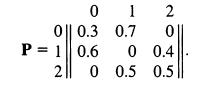
4.5. A Markov chain X,,, X,, X,, ... has the transition probability matrixA sojourn in a state is an uninterrupted sequence of consecutive visits to that state.(a) Determine the mean duration of a typical sojourn in state 0.(b) Using renewal theory, determine the long run fraction of time that the
4.4. A developing country is attempting to control its population growth by placing restrictions on the number of children each family can have.This society places a high premium on female children, and it is felt that any policy that ignores the desire to have female children will fail. The
4.3. Suppose that the life of a light bulb is a random variable X with hazard rate h(x) = Ox for x > 0. Each failed light bulb is immediately replaced with a new one. Determine an asymptotic expression for the mean age of the light bulb in service at time t, valid for t >> 0.
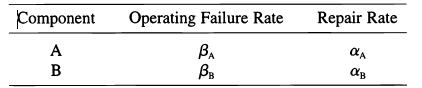
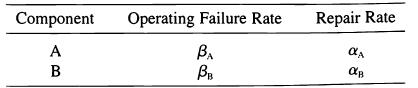
4.2. A system is subject to failures. Each failure requires a repair time that is exponentially distributed with rate parametera. The operating time of the system until the next failure is exponentially distributed with rate parameter /3. The repair times and the operating times are all
4.1. Suppose that a renewal function has the form M(t) = t +[1 - exp(-at)]. Determine the mean and variance of the interoccurrence distribution.
4.6. A machine can be in either of two states: "up" or "down." It is up at time zero and thereafter alternates between being up and down. The lengths X,, X,.... of successive up times are independent and identically distributed random variables with meana, and the lengths Y,, Y,, ... of successive
4.5. What is the limiting distribution of excess life when renewal lifetimes have the uniform density f(x) = 1, for 0 < x < 1?
4.4. Show that the optimal age replacement policy is to replace upon failure alone when lifetimes are exponentially distributed with parameter A. Can you provide an intuitive explanation?
4.3. Consider the triangular lifetime density function f(x) = 2x, for 0 < x < 1. Determine the optimal replacement age in an age replacement model with replacement cost K = 1 and failure penalty c = 4 (cf. the example in Section 4.1).
4.2. Consider the triangular lifetime density f(x) = 2x for 0 < x < 1.Determine an asymptotic expression for the probability distribution of excess life. Using this distribution, determine the limiting mean excess life and compare with the general result following equation (4.9).
4.1. Consider the triangular lifetime density f(x) = 2x for 0 < x < 1.Determine an asymptotic expression for the expected number of renewals up to time t.Hint: Use equation (4.5).
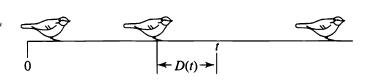
3.5. Birds are perched along a wire as shown according to a Poisson process of rate A per unit distanceAt a fixed point t along the wire, let D(t) be the random distance to the nearest bird. What is the mean value of D(t)? What is the probability density functionf(x) for D(t)? 0 -D(t)- D(t)
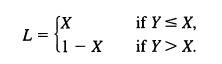
3.4. This problem is designed to aid in the understanding of lengthbiased sampling. Let X be a uniformly distributed random variable on[0, 1]. Then X divides [0, 1] into the subintervals [0, X] and (X, 1]. By symmetry, each subinterval has mean length ;. Now pick one of these subintervals at random
3.3. Pulses arrive at a counter according to a Poisson process of rate A.All physically realizable counters are imperfect, incapable of detecting all signals that enter their detection chambers. After a particle or signal arrives, a counter must recuperate, or renew itself, in preparation for the
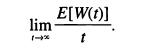
3.2. A fundamental identity involving the renewal function, valid for all renewal processes, isSee equation (1.7). Evaluate the left side and verify the identity when the renewal counting process is a Poisson process. E[W+]=E[X](M(t) + 1).
3.1. In another form of sum quota sampling (see V, Section 4.2), a sequence of nonnegative independent and identically distributed random variables X XZ, ... is observed, the sampling continuing until the first time that the sum of the observations exceeds the quota t. In renewal process
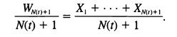
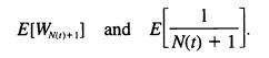
3.3. Let W,, W,, ... be the event times in a Poisson process (N(t); t ? 0)of rate A. Show that N(t) and WN(,)+I are independent random variables by evaluating Pr{N(t) = n and WN(,)+, > t + s).
3.2. Particles arrive at a counter according to a Poisson process of rate A. An arriving particle is recorded with probability p and lost with probability 1 - p independently of the other particles. Show that the sequence of recorded particles is a Poisson process of rate Ap.
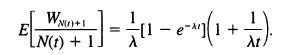
3.1. Let W,, W,, ... be the event times in a Poisson process (X(t); t ? 0)of rate A. Evaluate Pr{WN(,)+, > t + s} and E[WN(,)+I]
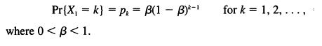
2.3. Determine M(n) when the interoccurrence times have the geometric distribution Pr{X =k} = p = (1 - B)*-1 where 0
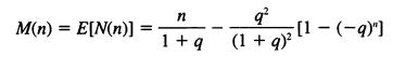
2.2. Let X,, X2, ... be the interoccurrence times in a renewal process.Suppose Pr(Xk = 1) = p and Pr{Xk = 2} = q = 1 - p. Verify thatforn=2,4,6..... n q M(n) =E[N(n)] [1-(-9)"] 1+9 (1 + q)
2.1. For the block replacement example of this section for which p, = 0.1, P2 = 0.4, p3 = 0.3, and p, = 0.2, suppose the costs arec, = 4 and c2 = 5. Determine the minimal cost block period K* and the cost of replacing upon failure alone.
2.3. Calculate the mean number of renewals M(n) = E[N(n)] for the renewal process having interoccurrence distribution for n = 1, 2, ... , 10. Also calculate u = M(n) - M(n - 1).
2.2. A certain type component has two states: 0 = OFF and 1 = OPERATING. In state 0, the process remains there a random length of time, which is exponentially distributed with parametera, and then moves to state 1. The time in state 1 is exponentially distributed with parameter 0, after which the

Showing 4600 - 4700 of 6914

First
40
41
42
43
44
45
46
47
48
49
50
51
52
53
54
Last

Step by Step Answers

Services

Sitemap
Fun
Definitions
Become Tutor
Used Textbooks
Study Help Categories
Recent Questions
Expert Questions
Campus Wear
Sell Your Books

Company Info

Security
Copyrights
Privacy Policy
Terms & Conditions
SolutionInn Fee
Scholarship
Online Quiz
Give Feedback, Get Rewards

Get In Touch

About Us
Contact Us
Career
Jobs
FAQ
Student Discount
Campus Ambassador

Secure Payment

Download Our App

© 2026 SolutionInn. All Rights Reserved