New Semester
Started
Get
50% OFF
Study Help!
--h --m --s
Claim Now
Question Answers
Textbooks
Find textbooks, questions and answers
Oops, something went wrong!
Change your search query and then try again
S
Books
FREE
Study Help
Expert Questions
Accounting
General Management
Mathematics
Finance
Organizational Behaviour
Law
Physics
Operating System
Management Leadership
Sociology
Programming
Marketing
Database
Computer Network
Economics
Textbooks Solutions
Accounting
Managerial Accounting
Management Leadership
Cost Accounting
Statistics
Business Law
Corporate Finance
Finance
Economics
Auditing
Tutors
Online Tutors
Find a Tutor
Hire a Tutor
Become a Tutor
AI Tutor
AI Study Planner
NEW
Sell Books
Search
Search
Sign In
Register
study help
business
statistical sampling to auditing
Introductory Probability And Statistical Applications 2nd Edition Paul L. Meyer - Solutions
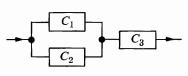
12.8. Suppose that the resistors in Problem 12.7 are connected in parallel. Find the pdf of R, the total resistance of the circuit (set up only, in integral form). [Hint: The relationship between R, and R1, and R2 is given by 1/R = 1/R1 + 1/R2.]
12.7. In a simple circuit two resistors R1 and R2 are connected in series. Hence the total resistance is given by R R + R2. Suppose that R and R2 are independent random variables each having the pdf f(ra) 10-ri 50 0 < r < 10, i = 1,2. Find the pdf of R, the total resistance, and sketch its graph.
12.6. Suppose that X, i = 1, 2,..., 50, are independent random variables each hav- ing a Poisson distribution with parameter =0.03. Let S = X++X50. (a) Using the Central Limit Theorem, evaluate P(S 3). (b) Compare the answer in (a) with the exact value of this probability.
12.5. A computer, in adding numbers, rounds each number off to the nearest inte- ger. Suppose that all rounding errors are independent and uniformly distributed over (-0.5, 0.5). (a) If 1500 numbers are added, what is the probability that the magnitude of the total error exceeds 15? (b) How many
12.4. Suppose that 30 electronic devices, say D1, ..., Dao, are used in the following manner: As soon as D fails D becomes operative. When D2 fails D3 becomes opera- tive, etc. Assume that the time to failure of D; is an exponentially distributed random variable with parameter 3 = 0.1 hour-1. Let T
12.3. (a) A complex system is made up of 100 components functioning independently. The probability that any one component will fail during the period of operation equals 0.10. In order for the entire system to function, at least 85 of the components must be working. Evaluate the probability of
12.2. Suppose that a sample of size n is obtained from a very large collection of bolts, 3 percent of which are defective. What is the probability that at most 5 percent of the chosen bolts are defective if: (a) n = 6? (b) n = 60? (c) n = 600?
12.1. (a) Items are produced in such a manner that 2 percent turn out to be defective. A large number of such items, say n, are inspected and the relative frequency of defec- tives, say fp, is recorded. How large should n be in order that the probability is at least 0.98 that fp differs from 0.02
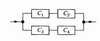
11.25. Consider the same system as described in Problem 11.24 except that this time components C1 and C3 fail together. Answer the questions of Problem 11.24.
11.23. If T, the time to failure of component C, is exponentially distributed with parameter B., obtain the reliability R(t) of the entire system. Also obtain the pdf of T, the time to failure of the system.
11.24. Consider four components C1, C2, C3, and C4 hooked up as indicated in Fig. 11.13. Suppose that the components function independently of one another with the exception of C1 and C2 which always fail together as described in Problem
11.23. Whenever we have considered a system made up of several components, we have always supposed that the components function independently of one another. This assumption has simplified our calculations considerably. However, it may not always be a realistic assumption. In many cases it is known
mgf.
11.22. Suppose that two independently functioning components, each with the same constant failure rate are connected in parallel. If 7 is the time to failure of the resulting system, obtain the mgf of T. Also determine E(T) and V(T), using the
11.21. Component A has reliability 0.9 when used for a particular purpose. Com- ponent B which may be used in place of component A has a reliability of only 0.75. What is the minimum number of components of type B that would have to be hooked up in parallel in order to achieve the same reliability
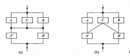
11.20. If all the components considered in Problem 11.19 have the same constant failure rate A, obtain an expression for the reliability R(t) for the system indicated in Fig. 11.12(b). Also find the mean time to failure of this system.
11.19. Consider components A, A', B, B', and C connected as indicated in Figs. 11.12 (a) and (b). (Component C may be thought of as representing a "safeguard" should both A and B fail to function.) Letting RA, RA', RB, RB', and Rc represent the reliabilities of the individual components (and
11.18. (a) An aircraft propulsion system consists of three engines. Assume that the constant failure rate for each engine is = 0.0005 and that the engines fail independently of one another. The engines are connected in parallel. What is the reliability of this propulsion system for a mission
11.17. Suppose that n components, each having the same constant failure rate \, are connected in parallel. Find an expression for the mean time to failure of the resulting system.
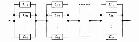
11.16. Suppose that k components are connected in parallel. Then n such parallel connections are hooked up in series into a single system. (See Figure 11.11.) Answer (a) and (b) of Problem 11.15 for this situation. Cin C12 C2n C22 C21 Ckl C12 Ckn
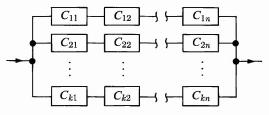
11.15. (a) Suppose that a components are hooked up in a series arrangement. Then k such series connections are hooked up in parallel to form an entire system. (See Figure 11.10.) If each component has the same reliability, say R, for a certain period of operation, find an expression for the
11.14. Suppose that each of three electronic devices has a failure law given by an exponential distribution with parameters 31, 32, and 83. Suppose that these three devices function independently and are connected in parallel to form a single system. (a) Obtain an expression for R(t), the
11.13. Suppose that the failure rate associated with the life length 7 of an item is given by the following function: Z(t) = Co, 0 1 < to, Co+C1(10), 1o. Note: This represents another generalization of the exponential distribution. The above reduces to constant failure rate (and hence the
11.12. (Taken from Derman and Klein, Probability and Statistical Inference. Oxford University Press, New York, 1959.) The life length (L) in months of a certain vacuum tube used in radar sets has been found to be exponentially distributed with parameter = 2. In carrying out its preventive
11.11. Suppose that n independently functioning components are connected in a series arrangement. Assume that the time to failure for each component is normally distributed with expectation 50 hours and standard deviation 5 hours. (a) If n 4, what is the probability that the system will still be
11.10. Three independently functioning components are connected into a single system as indicated in Fig. 11.9. Suppose that the reliability for each of the components for an operational period of hours is given by R(t) = 0.03 If T is the time to failure of the entire system (in hours), what is the
11.9. The life length of a satellite is an exponentially distributed random variable with expected life time equal to 1.5 years. If three such satellites are launched simul- taneously, what is the probability that at least two will still be in orbit after 2 years? C Cz FIGURE 11.9 11.10. Three
11.8. Prove Theorem 11.4.
11.7. Each of the six tubes of a radio set has a life length (in years) which may be considered as a random variable. Suppose that these tubes function independently of one another. What is the probability that no tubes will have to be replaced during the first two months of service if: (a) The pdf
11.6. Suppose that the failure law of a component is a linear combination of k exponential failure laws. That is, the pdf of the failure time is given by - f(t) ce 1>0, 8; > 0. (a) For what values of c; is the above a pdf? (b) Obtain an expression for the reliability function and hazard function.
11.5. Suppose that the failure law of a component has the following pdf: f(t) = (x + 1)A+/(A + 1)+2, 1 > 0. (a) For what values of A and r is the above a pdf? (b) Obtain an expression for the reliability function and hazard function. (c) Show that the hazard function is decreasing in 1.
11.4. Suppose that the failure rate Z is given by, Z(t) = 0, 0 < < A, = C, 1 A. (This implies that no failures occur before T = A.) (a) Find the pdf associated with T, the time to failure. (b) Evaluate E(T).
11.3. Suppose that the life length of a device has constant failure rate Co for 0 < t < to and a different constant failure rate C for 1 to. Obtain the pdf of T, the time to failure, and sketch it.
11.2. Suppose that the life length of an electronic device is exponentially distributed. It is known that the reliability of the device (for a 100-hour period of operation) is 0.90. How many hours of operation may be considered to achieve a reliability of 0.95?
11.1. Suppose that T, the time to failure, of an item is normally distributed with E(T) = 90 hours and standard deviation 5 hours. In order to achieve a reliability of 0.90, 0.95, 0.99, how many hours of operation may be considered?
10.20. A certain industrial process yields a large number of steel cylinders whose lengths are distributed normally with mean 3.25 inches and standard deviation 0.05 inch. If two such cylinders are chosen at random and placed end to end, what is the probability that their combined length is less
10.19. Find the mgf of a random variable which is uniformly distributed over (-1,2).
10.18. If the random variable X has an mgf given by Mx(t) standard deviation of X. = 3/(31), obtain the
10.17. Obtain the mgf of a random variable having a geometric distribution. Does this distribution possess a reproductive property under addition?
10.16. (The Poisson and the multinomial distribution.) Suppose that X, i = 1, 2,...,n are independently distributed random variables having a Poisson distribution with param- etersa, i = 1,...,n. Let X = X. Then the joint conditional probability distribution of X1,..., X, given X = x is given by a
10.15. Show that if X, i = 1, 2,..., k, represents the number of successes in ni repetitions of an experiment, where P(success) = p, for all i, then X ++ X has a binomial distribution. (That is, the binomial distribution possesses the reproductive property.)
10.14. Suppose that X1,..., X80 are independent random variables, each having distribution N(0, 1). Evaluate P[X++ Xo>77]. [Hint: Use Theorem 9.2.]
10.13. Suppose that the life length of an item is exponentially distributed with param- eter 0.5. Assume that 10 such items are installed successively, so that the ith item is installed "immediately" after the (i-1)-item has failed. Let T; be the time to failure of the ith item, i = 1, 2,..., 10,
10.12. Suppose that V, the velocity (cm/sec) of an object, has distribution N(0, 4). If KmV2/2 ergs is the kinetic energy of the object (where m = mass), find the pdf of K. If m 10 grams, evaluate P(K < 3).
10.11. If X has distribution X, using the mgf, show that E(X) = n and V(X) = 2n.
10.10. In a circuit n resistances are hooked up into a series arrangement. Suppose that each resistance is uniformly distributed over [0, 1] and suppose, furthermore, that all resistances are independent. Let R be the total resistance. (a) Find the mgf of R. (b) Using the mgf, obtain E(R) and V(R).
10.9. A number of resistances, R., i = 1, 2,..., n, are put into a series arrangement in a circuit. Suppose that each resistance is normally distributed with E(R.) = 10 ohms and V(R) = 0.16. (a) If n = 5, what is the probability that the resistance of the circuit exceeds 49 ohms? (b) How large
10.8. Suppose that the mgf of a random variable X is of the form Mx(1) (0.4e+0.6)8. (a) What is the mgf of the random variable Y = 3x + 2? (b) Evaluate E(X). (c) Can you check your answer to (b) by some other method? [Try to "recognize" Mx(t).]
10.7. Use the mgf to show that if X and Y are independent random variables with distribution N(z, 2) and N(, ), respectively, then Z = ax + bY is again normally distributed, where a and b are constants.
10.6. Suppose that the continuous random variable X has pdf f(x) = -1, (a) Obtain the mgf of X. (b) Using the mgf, find E(X) and V(X).
10.5. Find the mgf of the random variable X of Problem 6.7. Using the mgf, find E(X) and V(X).
10.4. Let X be the outcome when a fair die is tossed. (a) Find the mgf of X. (b) Using the mgf, find E(X) and V(X).
10.3. Suppose that X has the following pdf: f(x) = Ae-(-a), xa. (This is known as a two-parameter exponential distribution.) (a) Find the mgf of X. (b) Using the mgf, find E(X) and V(X).
10.2. (a) Find the mgf of the voltage (including noise) as discussed in Problem 7.25. (b) Using the mgf, obtain the expected value and variance of this voltage.
10.1. Suppose that X has pdf given by f(x) = 2x, 0 x 1. (a) Determine the mgf of X. (b) Using the mgf, evaluate E(X) and V(X) and check your answer. (See Note, p. 206.)
9.38. On the average a production process produces one defective item among every 300 manufactured. What is the probability that the third defective item will appear: (a) before 1000 pieces have been produced? (b) as the 1000th piece is produced? (c) after the 1000th piece has been produced? [Hint:
9.37. Assume that the number of accidents in a factory may be represented by a Poisson process averaging 2 accidents per week. What is the probability that (a) the time from one accident to the next will be more than 3 days, (b) the time from one accident to the third accident will be more than a
9.36. Suppose that a satellite telemetering device receives two kinds of signals which may be recorded as real numbers, say X and Y. Assume that X and Y are independent, continuous random variables with pdf's fand g, respectively. Suppose that during any specified period of time only one of these
9.35. In some tables for the normal distribution, H(x) = (1/2)fe-2/2 dt is tabulated for positive values of x (instead of (x) as given in the Appendix). If the random variable X has distribution N(1, 4) express each of the following probabilities in terms of tabulated values of the function H. (a)
9.34. Suppose that X, is defined as in Problem 9.33 with 8 = 30. What is the prob- ability that the time between successive emissions will be >5 minutes? >10 minutes? < 30 seconds?
9.33. Let X, be the number of particles emitted in hours from a radioactive source and suppose that X, has a Poisson distribution with parameter t. Let T equal the num- ber of hours until the first emission. Show that T has an exponential distribution with parameter . [Hint: Find the equivalent
9.32. Suppose that X has distribution N(0, 25). Evaluate P(1 < x < 4).
9.31. The annual rainfall at a certain locality is known to be a normally distributed random variable with mean value equal to 29.5 inches and standard deviation 2.5 inches. How many inches of rain (annually) is exceeded about 5 percent of the time?
9.30. Suppose that X, the length of a rod, has distribution N(10, 2). Instead of meas- uring the value of X, it is only specified whether certain requirements are met. Specifi- cally, each manufactured rod is classified as follows: X < 8,8 x < 12, and X 12. If 15 such rods are manufactured, what is
9.29. Suppose that a normally distributed random variable with expected value and variance 2 is truncated to the left at X = r and to the right at X = Y. Find the pdf of this "doubly truncated" random variable.
9.28. (a) Find the probability distribution of a binomially distributed random vari- able (based on n repetitions of an experiment) truncated to the right at X = n; that is, Xn cannot be observed. (b) Find the expected value and variance of the random variable described in (a).
9.27. Suppose that X has an exponential distribution truncated to the left as given by Eq. (9.24). Obtain E(X).
tabulated functions.
9.24. Suppose that V, the velocity (cm/sec) of an object having a mass of 1 kg, is a random variable having distribution N(0, 25). Let K = 1000V2/2 500 represent the kinetic energy (KE) of the object. Evaluate P(K < 200), P(K> 800). 9.25. Suppose that X has distribution N(u, 2). Using Theorem 7.7,
9.23. Suppose that the random variable X has a chi-square distribution with 10 de- grees of freedom. If we are asked to find two numbers a and b such that P(a < x
9.22. Prove Theorem 9.4.
9.21. Prove Theorem 9.3.
9.20. Verify the expressions for E(X) and V(X), where X has a Gamma distribution [see Eq. (9.18)].
9.19. Show that I)=. (See 9.15.) [Hint: Make the change of variable x u2/2 in the integral (4) fox-1/2e-* dx.]
9.18. Consider Example 9.8. Suppose that the operator is paid C3 dollars/hour while the machine is operating and C4 dollars/hour (C4 < C3) for the remaining time he has been hired after the machine has failed. Again determine for what value of H (the num- ber of hours the operator is being hired),
9.17. A rocket fuel is to contain a certain percent (say X) of a particular compound. The specifications call for X to be between 30 and 35 percent. The manufacturer will make a net profit on the fuel (per gallon) which is the following function of X: T(X) = $0.10 per gallon = $0.05 per gallon if
9.16. Let X1 and X2 be independent random variables each having distribution Nu, 2). Let Z(t) = X cos wt + X2 sin cof. This random variable is of interest in the study of random signals. Let V(t) = dZ(t)/dt. (w is assumed to be constant.) (a) What is the probability distribution of Z(t) and V(t)
9.15. Suppose that X, the breaking strength of rope (in pounds), has distribution N(100, 16). Each 100-foot coil of rope brings a profit of $25, provided X > 95. If X95, the rope may be used for a different purpose and a profit of $10 per coil is realized. Find the expected profit per coil.
9.14. Suppose that X is a random variable for which E(X) and V(X) = . Suppose that Y is uniformly distributed over the interval (a, b). Determine a and b so that E(X) = E(Y) and V(X) = V(Y).
9.13. Compare the upper bound on the probability P[|X - E(X) 2/V(X)] ob- tained from Chebyshev's inequality with the exact probability in each of the following cases. (a) X has distribution N(, ).(b) X has Poisson distribution with parameter A. (c) X has exponential distribution with parameter a.
9.12. The outside diameter of a shaft, say D, is specified to be 4 inches. Consider D to be a normally distributed random variable with mean 4 inches and variance 0.01 inch2. If the actual diameter differs from the specified value by more than 0.05 inch but less than 0.08 inch, the loss to the
9.11. Suppose that temperature (measured in degrees centigrade) is normally dis- tributed with expectation 50 and variance 4. What is the probability that the tempera- ture I will be between 48 and 53 centigrade?
9.10. Suppose that X has distribution N(u, 2). Determine c (as a function of and ) such that P(Xc) = 2P(X > c).
9.9. A distribution closely related to the normal distribution is the lognormal dis- tribution. Suppose that X is normally distributed with mean and variance o. Let Y = ex. Then Y has the lognormal distribution. (That is, Y is lognormal if and only if In Y is normal.) Find the pdf of Y. Note: The
9.8. Find the pdf of the random variable Q = X/Y, where X and Y are distributed as in Problem 9.7. (The distribution of Q is known as the Cauchy distribution.) Can you compute E(Q)?
9.7. Suppose that we are measuring the position of an object in the plane. Let X and Y be the errors of measurement of the x- and y-coordinates, respectively. Assume that X and Y are independently and identically distributed, each with distribution N(0, 2). Find the pdf of R = x2+ Y2. (The
9.6. We may be interested only in the magnitude of X, say Y = |X|. If X has dis- tribution N(0, 1), determine the pdf of Y, and evaluate E(Y) and V(Y).
9.5. Suppose that the life lengths of two electronic devices, say D1 and D2, have dis- tributions N(40, 36) and N(45, 9), respectively. If the electronic device is to be used for a 45-hour period, which device is to be preferred? If it is to be used for a 48-hour period, which device is to be
9.4. The errors in a certain length-measuring device are known to be normally dis- tributed with expected value zero and standard deviation 1 inch. What is the prob- ability that the error in measurement will be greater than 1 inch? 2 inches? 3 inches?
9.3. Suppose that the cable in Problem 9.2 is considered defective if the diameter dif- fers from its mean by more than 0.025. What is the probability of obtaining a defective cable?
9.2. The diameter of an electric cable is normally distributed with mean 0.8 and variance 0.0004. What is the probability that the diameter will exceed 0.81 inch?
9.1. Suppose that X has distribution N(2, 0.16). Using the table of the normal dis- tribution, evaluate the following probabilities. (a) P(X 2.3) (b) P(1.8x2.1)
8.25. With X and Y defined as in Section 8.6, prove or disprove the following: P(Y r).
8.24. Consider again the situation described in Problem 8.22. Suppose that each launching attempt costs $5000. In addition, a launching failure results in an additional cost of $500. Evaluate the expected cost for the situation described.
8.23. In the situation described in Problem 8.22, suppose that launching attempts are made until three consecutive successful launchings occur. Answer the questions raised in the previous problem in this case.
8.22. The probability of a successful rocket launching equals 0.8. Suppose that launching attempts are made until 3 successful launchings have occurred. What is the probability that exactly 6 attempts will be necessary? What is the probability that fewer than 6 attempts will be required?
8.21. Suppose that X, the number of particles emitted in hours from a radioactive source, has a Poisson distribution with parameter 201. What is the probability that ex- actly 5 particles are emitted during a 15-minute period?
8.20. The number of particles emitted from a radioactive source during a specified period is a random variable with a Poisson distribution. If the probability of no emissions equals, what is the probability that 2 or more emissions occur?
8.19. Prove Theorem 8.6.
8.18. Prove Theorem 8.4.
Showing 500 - 600
of 4976
1
2
3
4
5
6
7
8
9
10
11
12
13
14
15
Last
Step by Step Answers