New Semester Started Get 50% OFF Study Help! --h --m --s Claim Now

Question Answers

Textbooks

Find textbooks, questions and answers

Oops, something went wrong!

Change your search query and then try again

Result Not Found

Books FREE
Study Help
Tutors
AI Study Planner NEW
Sell Books

Search
Sign In
Register

study help
business
systems analysis and design using matlab

Design And Analysis Of Experiments 8th Edition Douglas C. Montgomery - Solutions

14.25. Consider the experiment described in Example 14.4.Demonstrate how the order in which the treatment combinations are run would be determined if this experiment were run as (a) a split-split-plot, (b) a split-plot, (c) a factorial design in a randomized block, and (d) a completely randomized
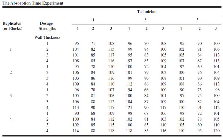
14.24. Suppose that in Problem 14.22 four technicians had been used. Assuming that all the factors are fixed, how many blocks should be run to obtain an adequate number of degrees of freedom on the test for differences among technicians? The Absorption Time Experiment Replicates (or Blocks) Dosage
14.23. Rework Problem 14.22, assuming that the technicians are chosen at random. Use the restricted form of the mixed model.
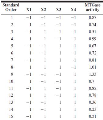
14.22. Consider the split-split-plot design described in Example 14.4. Suppose that this experiment is conducted as described and that the data shown in Table P14.3 are obtained.Analyze the data and draw conclusions.
14.21. Repeat Problem 14.20, assuming that the mixes are random and the application methods are fixed.
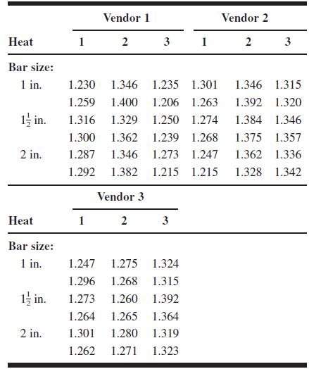
14.18. Suppose that in Problem 14.16 the bar stock may be purchased in many sizes and that the three sizes actually used in the experiment were selected randomly. Obtain the expected mean squares for this situation and modify the previous analysis appropriately. Use the restricted form of the mixed
14.17. Rework Problem 14.16 using the unrestricted form of the mixed model. You may use a computer software package to do this. Comment on any differences between the restricted and unrestricted model analysis and conclusions.
14.16. A structural engineer is studying the strength of aluminum alloy purchased from three vendors. Each vendor submits the alloy in standard-sized bars of 1.0, 1.5, or 2.0 inches. The processing of different sizes of bar stock from a common ingot involves different forging techniques, and so
14.15. Reanalyze the experiment in Problem 14.14 assuming the unrestricted form of the mixed model. You may use a computer software package to do this. Comment on any differences between the restricted and unrestricted model analysis and conclusions.
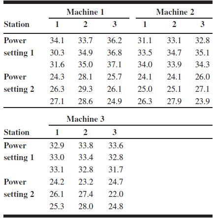
14.14. Suppose that in Problem 14.13 a large number of power settings could have been used and that the two selected for the experiment were chosen randomly. Obtain the expected mean squares for this situation assuming the restricted form of the mixed model and modify the previous analysis
14.13. A process engineer is testing the yield of a product manufactured on three machines. Each machine can be operated at two power settings. Furthermore, a machine has three stations on which the product is formed. An experiment is conducted in which each machine is tested at both power
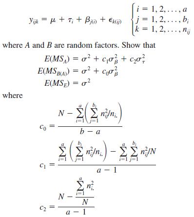
14.12. Variance components in the unbalanced two-stage nested design. Consider the model = Yijk Tj(i) + k (ij) i = 1, 2,..., a j = 1, 2,..., b k = 1, 2,..., nij where A and B are random factors. Show that where E(MSA) = + c + E(MSB(A)) =2+ co Co E(MSE) = b - / N- j=1 b-a b N N- a-1 n - a-1
14.10. Verify the expected mean squares given in Table 14.1.
14.9. Derive the expected mean squares for a balanced three-stage nested design if all three factors are random.Obtain formulas for estimating the variance components.
14.8. Repeat Problem 14.7 assuming the unrestricted form of the mixed model. You may use a computer software package to do this. Comment on any differences between the restricted and unrestricted model analysis and conclusions.
14.6. Reanalyze the experiment in Problem 14.5 using the unrestricted form of the mixed model. Comment on any differences you observe between the restricted and the unrestricted model results. You may use a computer software package.
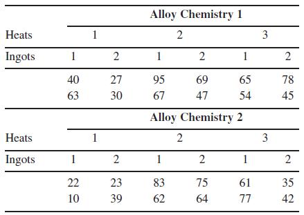
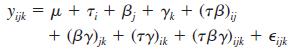
14.5. Consider the three-stage nested design shown in Figure 14.5 to investigate alloy hardness. Using the data that follow, analyze the design, assuming that alloy chemistry and heats are fixed factors and ingots are random. Use the restricted form of the mixed model. Heats 1 Alloy Chemistry 1 2 3
13.35. Rework Problem 13.31 using REML. Compare all sets of CIs for the variance components.
13.34 Consider the experiment in Problem 13.1. Analyze the data using REML. Compare the CIs to those obtained in Problem 13.28
13.33 Consider the experiment described in Problem 5.8.Estimate the variance components using the REML method.Compare the confidence intervals to the approximate CIs found in Problem 13.29
13.32. Rework Problem 13.28 using the modified largesample method described in Section 13.7.2. Compare this confidence interval with the one obtained previously and discuss.
13.31. Rework Problem 13.26 using the modified largesample approach described in Section 13.7.2. Compare the two sets of confidence intervals obtained and discuss.
13.30. Consider the three-factor experiment in Problem 5.19 and assume that operators were selected at random. Find an approximate 95 percent confidence interval on the operator variance component.
13.29. Use the experiment described in Problem 5.8 and assume that both factors are random. Find an exact 95 percent confidence interval on !2. Construct approximate 95 percent confidence intervals on the other variance components using the Satterthwaite method.
13.28. Consider the variance components in the random model from Problem 13.1.(a) Find an exact 95 percent confidence interval on !2.(b) Find approximate 95 percent confidence intervals on the other variance components using the Satterthwaite method.
13.27. Consider the two-factor mixed model. Show that the standard error of the fixed factor mean (e.g., A) is [MSAB/bn]1/2.
13.26. Analyze the data in Problem 13.1, assuming that operators are fixed, using both the unrestricted and the restricted forms of the mixed models. Compare the results obtained from the two models.
13.24. Show that the method of analysis of variance always produces unbiased point estimates of the variance components in any random or mixed model.
13.23. In the two-factor mixed model analysis of variance, show that Cov[(.")ij, (.")i6j] $ !(1/a) for i @ i6.
13.22. In Problem 5.8, assume that both machines and operators were chosen randomly. Determine the power of the test for detecting a machine effect such that $ !2, where is the variance component for the machine factor. Are two replicates sufficient?
13.21. The three-factor factorial model for a single replicate isIf all the factors are random, can any effects be tested? If the three-factor and (.")ij interactions do not exist, can all the remaining effects be tested? Yijk +T; + B; + Yk + (TB) ij +(BY)jk + (TY)ik + (TBY)ijk + Eijk
13.20. Consider the three-factor factorial modelAssuming that all the factors are random, develop the analysis of variance table, including the expected mean squares. Propose appropriate test statistics for all effects. Yijk +T+B; + Yk + (TB)ij i = 1, 2,..., a +(BY)jk + Eijk j = 1, 2,..., b k = 1,
13.19. In Problem 5.19, assume that the three operators were selected at random. Analyze the data under these conditions and draw conclusions. Estimate the variance components.
13.18. Reconsider cases (c), (d), and (e) of Problem 13.17.Obtain the expected mean squares assuming the unrestricted model. You may use a computer package such as Minitab. Compare your results with those for the restricted model.
13.16. Derive the expected mean squares shown in Table 13.11.
13.15. Consider the experiment in Example 13.6. Analyze the data for the case where A, B, and C are random.
13.14. Consider the three-factor factorial design in Example 13.5. Propose appropriate test statistics for all main effects and interactions. Repeat for the case where A and B are fixed and C is random.
13.13. By application of the expectation operator, develop the expected mean squares for the two-factor factorial, mixed model. Use the restricted model assumptions. Check your results with the expected mean squares given in Equation 13.9 to see that they agree.
13.12 Rework Problem 13.8 using the REML method.
13.11 Rework Problem 13.7 using the REML method.
13.10 Rework Problem 13.6 using the REML method.
13.9 Rework Problem 13.5 using the REML method.
13.8. In Problem 5.8, suppose that there are only four machines of interest, but the operators were selected at random.(a) What type of model is appropriate?(b) Perform the analysis and estimate the model components using the ANOVA method.
13.7. Reanalyze the measurement system experiment in Problem 13.2, assuming that operators are a fixed factor.Estimate the appropriate model components using the ANOVA method.
13.6. Reanalyze the measurement systems experiment in Problem 13.1, assuming that operators are a fixed factor.Estimate the appropriate model components using the ANOVA method.
13.5. Suppose that in Problem 5.13 the furnace positions were randomly selected, resulting in a mixed model experiment.Reanalyze the data from this experiment under this new assumption. Estimate the appropriate model components using the ANOVA method.
13.4. Reconsider the data in Problem 5.15. Suppose that both factors are random.(a) Analyze the data from this experiment.(b) Estimate the variance components using the ANOVA method.
13.3. Reconsider the data in Problem 5.8. Suppose that both factors, machines and operators, are chosen at random.(a) Analyze the data from this experiment.(b) Find point estimates of the variance components using the analysis of variance method.
13.2. An article by Hoof and Berman (“Statistical Analysis of Power Module Thermal Test Equipment Performance,”IEEE Transactions on Components, Hybrids, and Manufacturing Technology Vol. 11, pp. 516–520, 1988)describes an experiment conducted to investigate the capability of measurements in
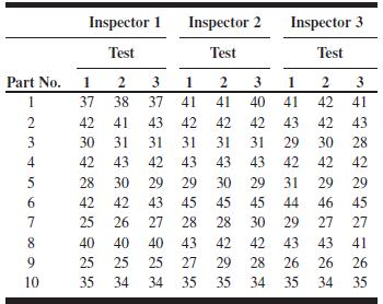
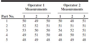
13.1. An experiment was performed to investigate the capability of a measurement system. Ten parts were randomly selected, and two randomly selected operators measured each part three times. The tests were made in random order, and the data are shown in Table P13.1.(a) Analyze the data from this
12.21. Consider the alloy cracking experiment in Problem 6.15. Suppose that temperature (A) is a noise variable. Find the response model, and the model for the mean response, and the model for the transmitted variability. Can you find settings for the controllable factors that minimize crack length
12.20. Reconsider the wave soldering experiment in Problem 12.16. Suppose that it was necessary to fit a complete quadratic model in the controllable variables, all main effects of the noise variables, and all controllable variable–noise variable interactions. What design would you recommend?
12.19. Reconsider the wave soldering experiment in Problem 12.16. Find a combined array design for this experiment that requires fewer runs.
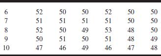
12.18. An experiment was run in a wave soldering process.There are five controllable variables and three noise variables.The response variable is the number of solder defects per million opportunities. The experimental design employed was the following crossed array.(a) What types of designs were
12.17. Rework Problem 12.12 using the I-criterion. Compare this design to the D-optimal design in Problem 12.12. Which design would you prefer?
12.16. Rework Problem 12.15 using the I-criterion to construct the design. Compare this design to the D-optimal design in Problem 12.15. Which design would you prefer?
12.15. Reconsider the situation in Problem 12.13. What is the minimum number of runs that can be used to estimate all of the model parameters using a combined array design? Use a Doptimal algorithm to find a reasonable design for this problem.
12.14. Reconsider the situation in Problem 12.13. Could a modified small composite design be used for this problem?Are any disadvantages associated with the use of the small composite design?
12.13. Suppose that there are four controllable variables and two noise variables. It is necessary to fit a complete quadratic model in the controllable variables, the main effects of the noise variables, and the two-factor interactions between all controllable and noise factors. Set up a combined
12.12. Suppose that there are four controllable variables and two noise variables. It is necessary to estimate the main effects and two-factor interactions of all of the controllable variables, the main effects of the noise variables, and the twofactor interactions between all controllable and
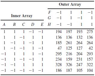
12.11. An experiment has been run in a process that applies a coating material to a wafer. Each run in the experiment produced a wafer, and the coating thickness was measured several times at different locations on the wafer. Then the mean y1 and the standard deviation y2 of the thickness
12.10. In an article (“Let’s All Beware the Latin Square,”Quality Engineering, Vol. 1, 1989, pp. 453–465), J. S. Hunter illustrates some of the problems associated with 3k!p fractional factorial designs. Factor A is the amount of ethanol added to a standard fuel, and factor B represents the
12.9. A variation of Example 12.1. In Example 12.1(which utilized data from Example 6.2), we found that one of the process variables (B $ pressure) was not important.Dropping this variable produces two replicates of a 23 design.The data are as follows:Assume that C and D are controllable factors
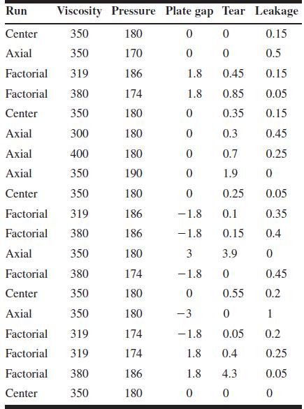
12.8. Consider the experiment in Problem 11.11. Suppose that pressure is a noise variable ( in coded units). Fit the response model for the viscosity response. Find a set of conditions that result in viscosity as close as possible to 600 and that minimize the variability transmitted from the noise
12.7. Consider the connector pull-off force experiment shown in Table 12.2. Show how an experiment can be designed for this problem that will allow a full quadratic model to be fit in the controllable variables along all main effects of the noise variables and their interactions with the
12.6. Consider the connector pull-off force experiment shown in Table 12.2. What main effects and interaction involving the controllable variables can be estimated with this design? Remember that all of the controllable variables are quantitative factors.
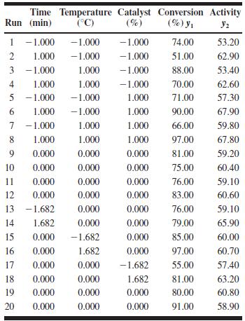
12.5. Continuation of Problem 12.5. Reconsider the leaf spring experiment from Table 12.1. Suppose that factors A, B and C are controllable variables and that factors D and E are noise factors. Show how a combined array design can be employed to investigate this problem that allows all twofactor
12.4. Reconsider the leaf spring experiment from Table 12.1. Suppose that factors A, B, and C are controllable variables and that factors D and E are noise factors. Set up a crossed array design to investigate this problem, assuming that all of the two-factor interactions involving the controllable
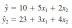
12.3. Consider the experiment in Problem 11.12. Suppose that temperature is a noise variable ( in coded units). Fit response models for both responses. Is there a robust design problem with respect to both responses? Find a set of conditions that maximize conversion with activity between 55 and 60
12.2. Consider the bottle-filling experiment in Problem 6.20. Suppose that the percentage of carbonation (A) is a noise variable ( in coded units).(a) Fit the response model to these data. Is there a robust design problem?(b) Find the mean model and either the variance model or the POE.(c) Find a
12.1. Reconsider the leaf spring experiment in Table 12.1.Suppose that the objective is to find a set of conditions where the mean free height is as close as possible to 7.6 inches, with the variance of free height as small as possible. What conditions would you recommend to achieve these
11.37. An article in the Electronic Journal of Biotechnology (“Optimization of Medium Composition for Transglutaminase Production by a Brazilian Soil Streptomyces sp,” available at http://www.ejbiotechnology.info/content/vol10/issue4/full/10.index.html) describes the use of designed experiments
11.36. An article in the Journal of Chromatography A(“Optimization of the Capillary Electrophoresis Separation of Ranitidine and Related Compounds,” Vol. 766, pp. 245–254)describes an experiment to optimize the production of ranitidine, a compound that is the primary active ingredient of
11.35. The Paper Helicopter Experiment Revisited.Reconsider the paper helicopter experiment in Problem 11.34.This experiment was actually run in two blocks. Block 1 consisted of the first 16 runs in Table P11.11 (standard order runs 1–16) and two center points (standard order runs 25 and 26).11.8
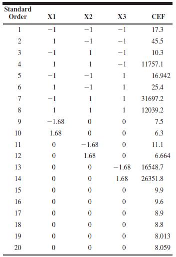
11.34. Box and Liu (1999) describe an experiment flying paper helicopters where the objective is to maximize flight time. They used the central composite design shown in Table P11.11. Each run involved a single helicopter made to the following specifications: x1 $ wing area (in2), !1 $ 11.80 and%1
11.33. An article in Quality Progress (“For Starbucks, It’s in the Bag,” March 2011, pp. 18–23) describes using a central composite design to improve the packaging of one-pound coffee. The objective is to produce an airtight seal that is easy to open without damaging the top of the coffee
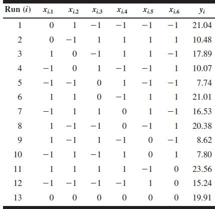
11.32. Table P11.9 shows a six-variable RSM design from Jones and Nachtsheim (2011b). Analyze the response data from this experiment. Run (i) Xi.1 Xi.2 Xi.3 Xi.A Xi.5 Xi.6 Yi 1 0 1 -1 -1 -1 -1 21.04 23 2 0 -1 1 1 1 1 10.48 10 -1 1 1 -1 17.89 4 T 0 1 1 10.07 5 -1 -1 0 1 -1 -1 7.74 6 11 0 -1 1 1
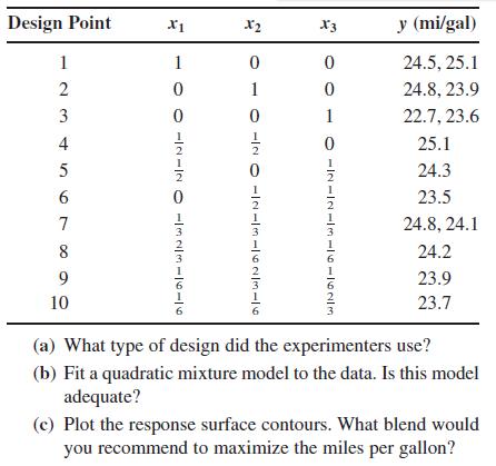
11.31. Myers, Montgomery and Anderson-Cook (2009)describe a gasoline blending experiment involving three mixture components. There are no constraints on the mixture proportions, and the following 10-run design is used: Design Point x1 x2 X3 y (mi/gal) 123 1 1 0 0 24.5, 25.1 2 0 1 0 24.8, 23.9 3 0 4
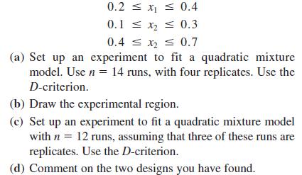
11.30. An experimenter wishes to run a three-component mixture experiment. The constraints in the component proportions are as follows: 0.2 x 0.4 0.12 0.3 0.4 x 0.7 (a) Set up an experiment to fit a quadratic mixture model. Use n = 14 runs, with four replicates. Use the D-criterion. (b) Draw the
11.29. Suppose that you want to fit a second-order response surface model in a situation where there are k $ 4 factors;however, one of the factors is categorical with two levels.What model should you consider for this experiment? Suggest an appropriate design for this situation.
11.28. Suppose that you want to fit a second-order model in k $ 5 factors. You cannot afford more than 25 runs. Construct both a D-optimal and on I-optimal design for this situation.Compare the prediction variance properties of the designs.Which design would you prefer?
11.27. Rework problem 11.26 assuming that the model the engineer wishes to fit is a quadratic. Obviously, only designs 2, 3, and 4 can now be considered.
11.25. Repeat problem 11.24 using a first-order model with the two-factor interactions.
11.24. Consider a 23 design for fitting a first-order model.(a) Evaluate the D-criterion (X6X)!1 for this design.(b) Evaluate the A-criterion tr(X6X)!1 for this design.(c) Find the maximum scaled prediction variance for this design. Is this design G-optimal?
11.22. Suppose that we approximate a response surface with a model of order d1, such as y $ X1&1 % >, when the true surface is described by a model of order d2 , d1; that is, E(y)$ X1&1 % X1&2.(a) Show that the regression coefficients are biased, that is, E $ &1 % A&2, where A $ . A is usually
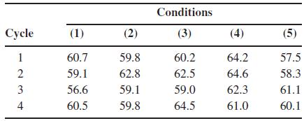
11.21. Yield during the first four cycles of a chemical process is shown in the following table. The variables are percentage of concentration (x1) at levels 30, 31, and 32 and temperature (x2)at 140, 142, and 144°F. Analyze by EVOP methods. Conditions Cycle (1) (2) (3) (4) (5) 1 60.7 59.8 60.2
11.20. How could a hexagon design be run in two orthogonal blocks?
11.19. Blocking in the central composite design. Consider a central composite design for k $ 4 variables in two blocks. Can a rotatable design always be found that blocks orthogonally?
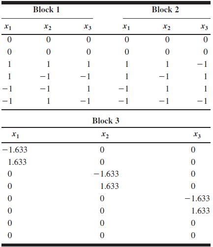
11.18. Verify that the central composite design shown in Table P11.8 blocks orthogonally: Block 1 Block 2 X1 x2 X3 x1 x2 X3 0 0 0 0 0 0 0 0 0 0 0 0 1 1 1 1 1 -1 1 1 1 1 -1 1 -1 -1 -1 -1 Block 3 x1 x2 X3 -1.633 0 0 1.633 0 0 0 -1.633 0 0 1.633 0 0 0 -1.633 0 0 1.633 0 0 0 0 0 0
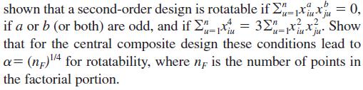
11.17. The rotatable central composite design. It can be shown that a second-order design is rotatable if a b x = 0, ju if a or b (or both) are odd, and if x = 3xx Show that for the central composite design these conditions lead to a= (n) 1/4 for rotatability, where n is the number of points in the
11.16. Show that augmenting a 2k design with nC center points does not affect the estimates of the "i (i $ 1, 2, . . . , k)but that the estimate of the intercept "0 is the average of all 2k% nc observations.
11.15. Verify that an orthogonal first-order design is also first-order rotatable.
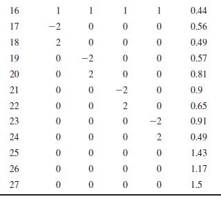
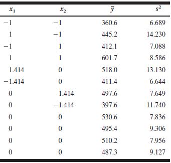
11.14. A central composite design is run in a chemical vapor deposition process, resulting in the experimental data shown in Table P11.7. Four experimental units were processed simultaneously on each run of the design, and the responses are the mean and the variance of thickness, computed across
11.13. A manufacturer of cutting tools has developed two empirical equations for tool life in hours (y1) and for tool cost in dollars (y2). Both models are linear functions of steel hardness(x1) and manufacturing time (x2). The two equations areand both equations are valid over the range !1.5 # xi
11.12. Consider the three-variable central composite design shown in Table P11.6. Analyze the data and draw conclusions, assuming that we wish to maximize conversion (y1) with activity (y2) between 55 and 60. Time Temperature Catalyst Conversion Activity Run (min) (C) (%) (%) Y 32 1 -1.000 -1.000
11.11. An experimenter has run a Box–Behnken design and obtained the results as shown in Table P11.5, where the response variable is the viscosity of a polymer:(a) Fit the second-order model.(b) Perform the canonical analysis. What type of surface has been found?(c) What operating conditions on
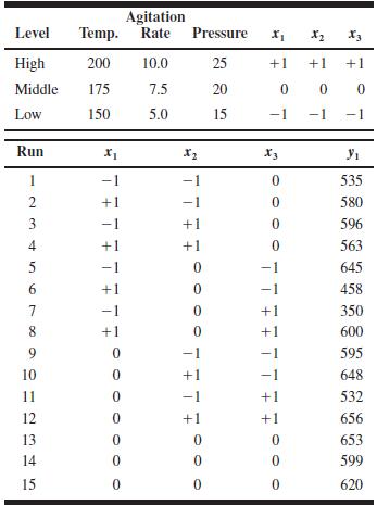
11.10. The hexagon design in Table P11.4 is used in an experiment that has the objective of fitting a second-order model:(a) Fit the second-order model.(b) Perform the canonical analysis. What type of surface has been found?(c) What operating conditions on x1 and x2 lead to the stationary point?(d)
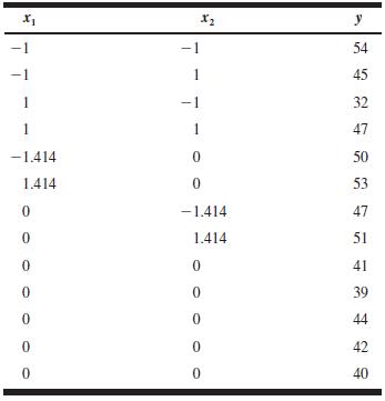
11.9. The data in Table P11.3 were collected by a chemical engineer. The response y is filtration time, x1 is temperature, and x2 is pressure. Fit a second-order model.(a) What operating conditions would you recommend if the objective is to minimize the filtration time?(b) What operating conditions
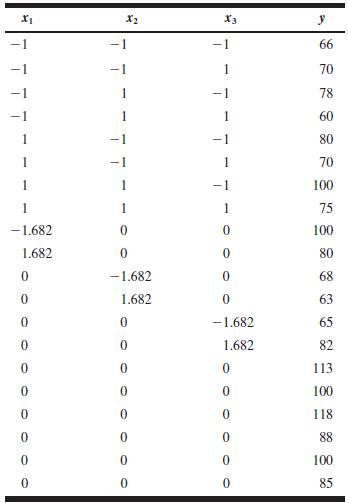
11.8. The data shown in the Table P11.2 were collected in an experiment to optimize crystal growth as a function of three variables x1, x2, and x3. Large values of y (yield in grams)are desirable. Fit a second-order model and analyze the fitted surface. Under what set of conditions is maximum
11.7. The path of steepest ascent is usually computed assuming that the model is truly first order; that is, there is no interaction. However, even if there is interaction, steepest ascent ignoring the interaction still usually produces good results. To illustrate, suppose that we have fit the

Showing 1500 - 1600 of 2697

First
9
10
11
12
13
14
15
16
17
18
19
20
21
22
23
Last

Step by Step Answers

Services

Sitemap
Fun
Definitions
Become Tutor
Used Textbooks
Study Help Categories
Recent Questions
Expert Questions
Campus Wear
Sell Your Books

Company Info

Security
Copyrights
Privacy Policy
Terms & Conditions
SolutionInn Fee
Scholarship
Online Quiz
Give Feedback, Get Rewards

Get In Touch

About Us
Contact Us
Career
Jobs
FAQ
Student Discount
Campus Ambassador

Secure Payment

Download Our App

© 2026 SolutionInn. All Rights Reserved