New Semester
Started
Get
50% OFF
Study Help!
--h --m --s
Claim Now
Question Answers
Textbooks
Find textbooks, questions and answers
Oops, something went wrong!
Change your search query and then try again
S
Books
FREE
Study Help
Expert Questions
Accounting
General Management
Mathematics
Finance
Organizational Behaviour
Law
Physics
Operating System
Management Leadership
Sociology
Programming
Marketing
Database
Computer Network
Economics
Textbooks Solutions
Accounting
Managerial Accounting
Management Leadership
Cost Accounting
Statistics
Business Law
Corporate Finance
Finance
Economics
Auditing
Tutors
Online Tutors
Find a Tutor
Hire a Tutor
Become a Tutor
AI Tutor
AI Study Planner
NEW
Sell Books
Search
Search
Sign In
Register
study help
computer science
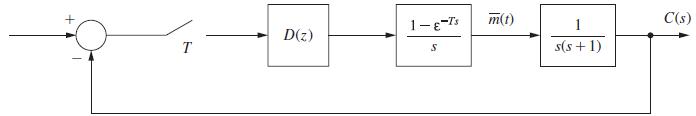
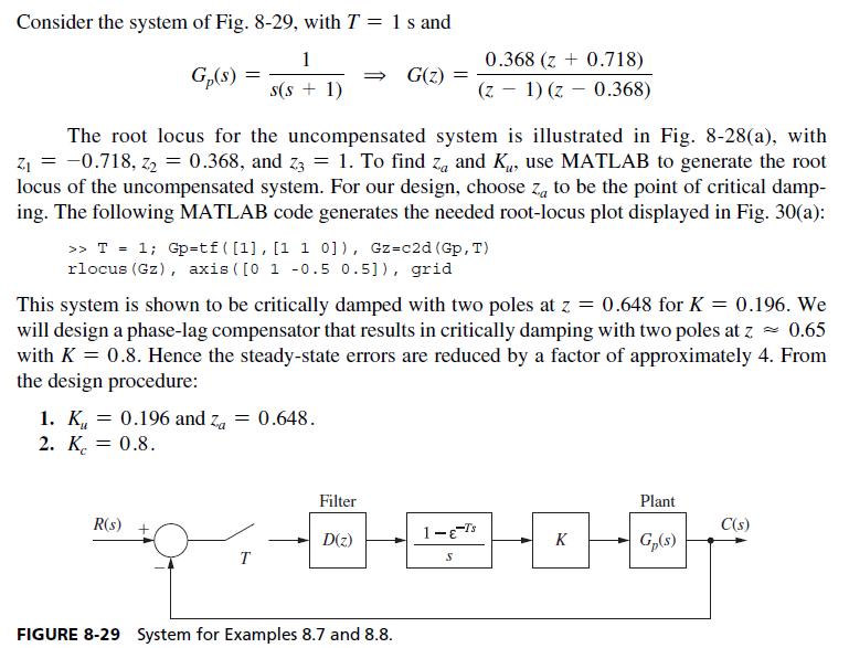
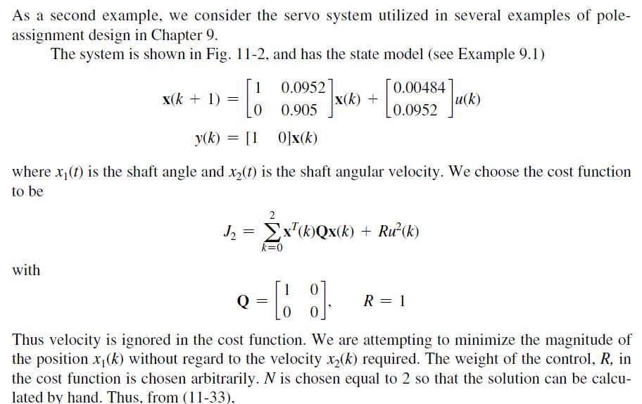
digital control system analysis and design
Digital Control System Analysis And Design 4th Edition Charles Phillips, H. Nagle, Aranya Chakrabortty - Solutions
If the rectangular integrator [see below (8-38)] is used in the PID transfer function in (8-52), the resulting controller is described by\[\frac{M(z)}{E(z)}=D(z)=K_{p}+K_{I}\left[\frac{T z}{z-1}ight]+K_{D}\left[\frac{z-1}{T z}ight]\]This transfer function is implemented in many commercial digital
Repeat Problem 8.6-2 using a proportional-plus-derivative (PD) filter.Problem 8.6-2Repeat Problem 8.4-2 using a phase-lead controller. In part (c), the overshoot is approximately 26 percent.Problem 8.4-2(c)(c) Verify the step-response results in part (b) using MATLAB. The step response will show
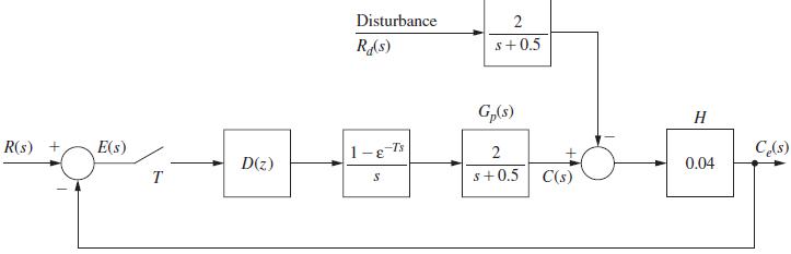
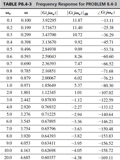
Repeat Problem 8.4-3 for a proportional-plus-integral (PI) compensator. Note that in this case, the steady-state error for a constant input is zero.Problem 8.4-3 Shown in Fig. P8.4-3 is the block diagram of the temperature control system described in Problem 1.6-1. For this problem, ignore the
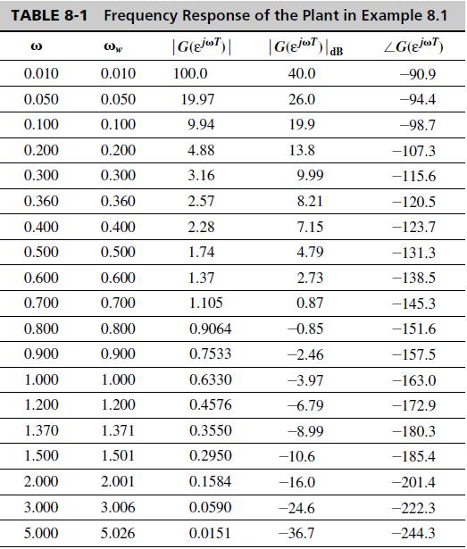
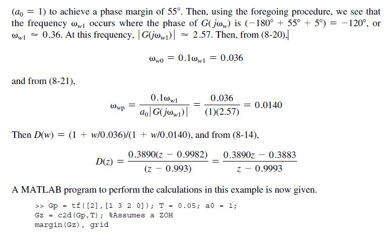
Consider the system of Example 8.1.(a) Design a PI filter to achieve a phase margin of \(60^{\circ}\).(b) Obtain the system step response using MATLAB. Compare this response to that of the system of Example 8.1, which is plotted in Fig. 8-14.Example 8.1We will consider the design of a servomotor
Consider the chamber temperature control system of Problem 8.4-3. Suppose that a variable gain \(K\) is added to the plant. The pulse transfer function for this system is given in Problem 8.4-3.(a) Plot the root locus for this system and find the value of \(K>0\) for which the system is
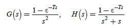
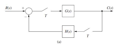
Consider the system of Fig. P8.2-2 with a gain factor KK added to the plant.(a) Show that the pulse transfer function is given by(b) Sketch the root locus for this system, and find the value of KK that results in critical damping, that is, in two real and equal roots of the system characteristic
Consider the system of Example 8.7.(a) Design a phase-lag compensator such that with \(K=0.5\), the system is critically damped with roots having a time constant of approximately \(2.03 \mathrm{~s}\). This time constant is the same as that of the uncompensated system with \(K=0.244\).(b) By
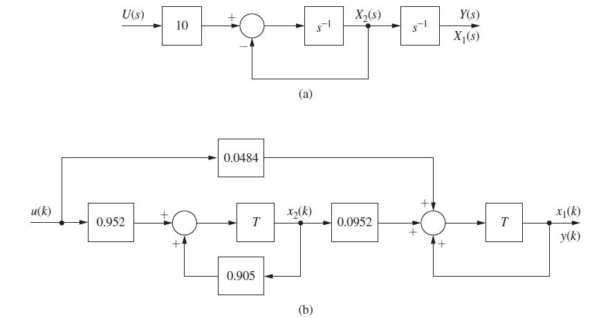
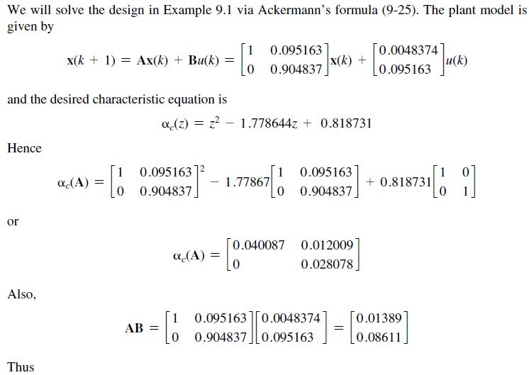
The plant of Example 9.1 has the state equations given (9-1). Find the gain matrix KK required to realize the closed-loop characteristic equation with zeros which have a damping ratio ζζ of 0.46 and a time constant ττ of 0.5 s0.5 s. Use pole-assignment design.Example 9.1Equation 9-1 As a
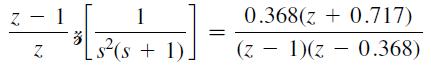
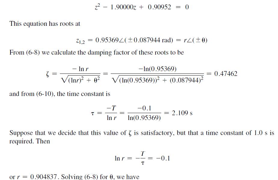
Consider the plant of Problem 9.2-1, which has the transfer function, from Example 9.5,G(z)=z−1zz[1s2(s+1)]=0.00484z+0.00468z2−1.905z+0.905G(z)=z−1zz[1s2(s+1)]=0.00484z+0.00468z2−1.905z+0.905(a) Using the pole-assignment design, find the gain matrix KK required to realize the closed-loop
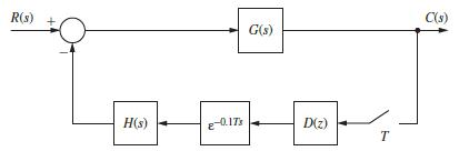
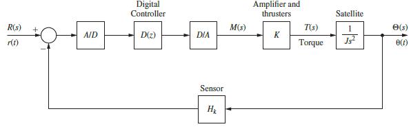
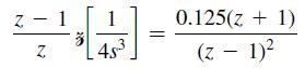
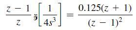
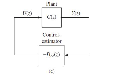
A satellite control system is modeled as shown in Fig. P9.2-4. This system is described in Problem 1.4-1. For this problem, let D(z)=1D(z)=1D(z)=1K=1,T=1 s,J=4. In addition, K=1,T=1 s,J=4Hk=1, and Hk=1z. From the zz−1zz[14s3]=0.125(z+1)(z−1)2-transform
Consider the pole-placement design of Problem 9.2-2.Problem 9.2-2Consider the plant of Problem 9.2-1, which has the transfer function, from Example 9.5,Problem 9.2-1The plant of Example 9.1 has the state equations given (9-1). Find the gain matrix K required to realize theclosed-loop characteristic
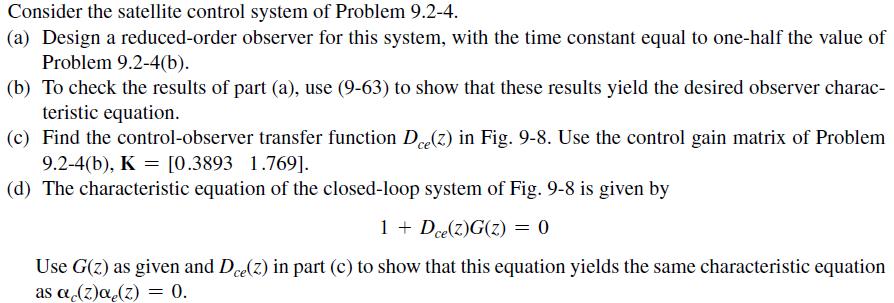
Consider the satellite control system of Problem 9.2-4.Problem 9.2-4A satellite control system is modeled as shown in Fig. P9.2-4. This system is described in Problem 1.4-1.For this problem, let D(z) = 1. In addition, K = 1, T = 1 s, J = 4, and Hk = 1. From the z-transformtables,(a) Design a
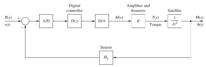
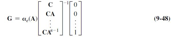
Assume that equation (9-25), Ackermann's formula for pole-assignment design, is the solution of (9-15). Based on this result, show that (9-48), Ackermann's formula for observer design, is the solution of (9-46).Equation 9-15Equation 9-25Equation 9-48Equation 9-46 a(z) = |zI = A + BK| = (z A)(z-
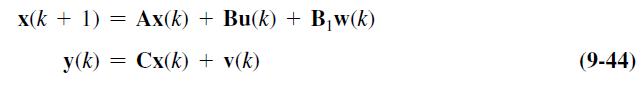
Given in (9-56) is the closed-loop state model for the pole-placement prediction-estimator design. Extend this model to include plant disturbances and sensor noise, as described in (9-44).Equation 9-56Equation 9-44 A B]= [Gc q(k+ 1). GC x(k+ 1) - BK x(k) BK ][ N(6)] AGC BK (9-56)
Consider the control system of Problem 9.2-2.Problem 9.2-2Consider the plant of Problem 9.2-1, which has the transfer function, from Example 9.5,Problem 9.2-1The plant of Example 9.1 has the state equations given (9-1). Find the gain matrix K required to realize theclosed-loop characteristic
Consider the satellite control system of Problem 9.2-4.Problem 9.2-4A satellite control system is modeled as shown in Fig. P9.2-4. This system is described in Problem 1.4-1.For this problem, let D(z) = 1. In addition, K = 1, T = 1 s, J = 4, and Hk = 1. From the z-transformtables,Fig. P9.2-4(a)
Consider the reduced-order observer designed in Problem 9.4-2. In this problem, velocity [dy/dt][dy/dt] is estimated, using position [y][y] plus other information. We could simply calculate velocity, using one of the numerical differentiators described in Section 8.8. This calculated velocity would
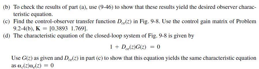
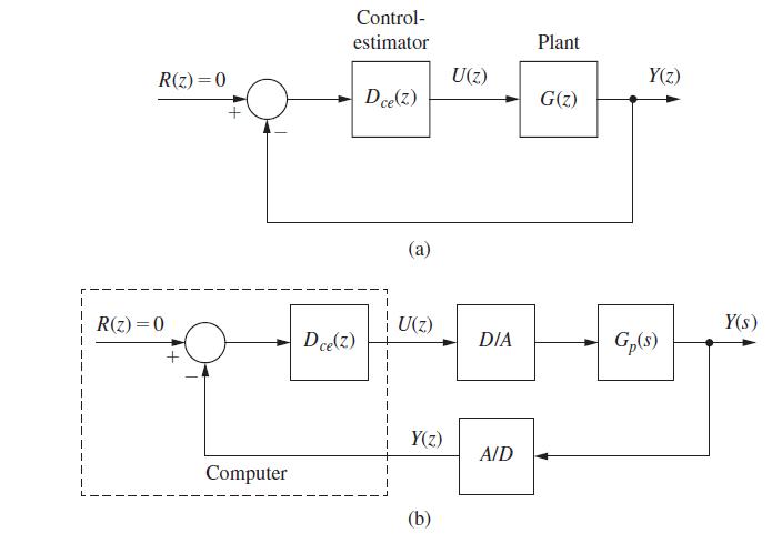
Consider that in Fig. 9-8, the observer is reduced order, and that the system is single-input single output. Show that the transfer function Dce(z)Dce(z) of the equivalent controller is given by.Fig. 9-8 R(z) =0 R(z)=0 + Computer Control- estimator Dce(z) Dce(z) (a) U(z) Y(z) (b) U(z) DIA A/D Plant
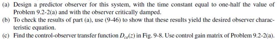
Repeat all parts of Problem 9.3-1 using a current observer.Problem 9.3-1 (a) Design a predictor observer for this system, with the time constant equal to one-half the value of Problem 9.2-2(a) and with the observer critically damped. (b) To check the results of part (a), use (9-46) to show that
Repeat all parts of Problem 9.3-2, using a current observer.Problem 9.3-2 (a) Design a predictor observer for this system, with the time constant equal to one-half the value of Problem 9.2-3(b). (b) To check the results of part (a), use (9-46) to show that these results yield the desired observer
(a) Find the closed-loop state equations for the system of Problem 9.3-2(a), of the form of (9-56).(b) Find the system characteristic equation using the results in part (a), and show that this is the desired equation.(c) Repeat parts (a) and (b) for the closed-loop system of Problem 9.5-2.Problem
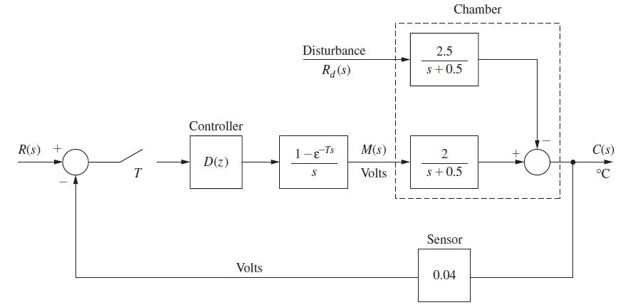
Consider the chamber temperature control system of Fig. P9.2-3. For this problem, replace the sensor gain \(H=0.04\) with the gain \(H=1\). The system is now a unity-gain feedback system.(a) Work Problem 9.2-3 with \(H=1\).(b) Work Problem 9.3-2 with \(H=1\).(c) Work Problem 9.5-2 with \(H=1\).(d)
Repeat all parts of Problem 9.3-3, using a current observer.Problem 9.3-3 (a) Design a predictor observer for this system, with the time constant equal to one-half the value of Problem 9.2-4(b) and with the observer critically damped.
(a) Show that for the current observer specified in Section 9.5, the transfer matrix from the input \(\mathbf{U}(z)\) to the estimated states \(\mathbf{Q}(z)\) is equal to that from the input to the states \(\mathbf{X}(z)\); that is, show that \(\mathbf{Q}(z) / \mathbf{U}(z)=\mathbf{X}(z) /
Derive the closed-loop state model for the pole-placement current-estimator design, given in (9-74). B] =[GCA x(k+ q(k+ 1). -BK A - GCA x(k) BKq(k) (9-74)
Consider a system described by (9-82).Equations 9-82For the case that u(k) is not zero, derive the conditions for observability. x(k+ 1) = Ax(k) + Bu(k) y(k) Cx(k) =
Consider the plant of Example 9.2, which is(a) Is this system observable?(b) Explain the reason for your answer in part (a) in terms of the physical aspects of the system.Example 9.2 x(k + 1) = Suppose that the output is given by 1 0.0952 0.9048] x(k) + y(k) = [0 1]x(k) 0.00484 0.0952u(k)
Consider the satellite control system of Problem 9.2-4. Suppose that the output is the measurement of angular velocity, such that(a) Is this system observable?(b) Explain your answer in part (a) in terms of the physical aspects of the system. We are attempting to estimate position, given
Consider the first-order plant described byand a prediction observer described by (9-38).(a) Construct a single set of state equations for the plant-observer system, with the state vector [x(k)q(k)T][x(k)q(k)T] and the input u(k)u(k) (i.e., there is no feedback).(b) Show that this system is always
Problem 9.6-7 is to be repeated for the current observer, with the mode of Q(z)Q(z) equal to (A−GCA)k(A−GCA)k.Problem 9.6-7For the system of Problem 9.6-5, use a transfer function approach to show that the transfer function Q(z)/U(z) is first order (even though the system is second order) and
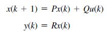
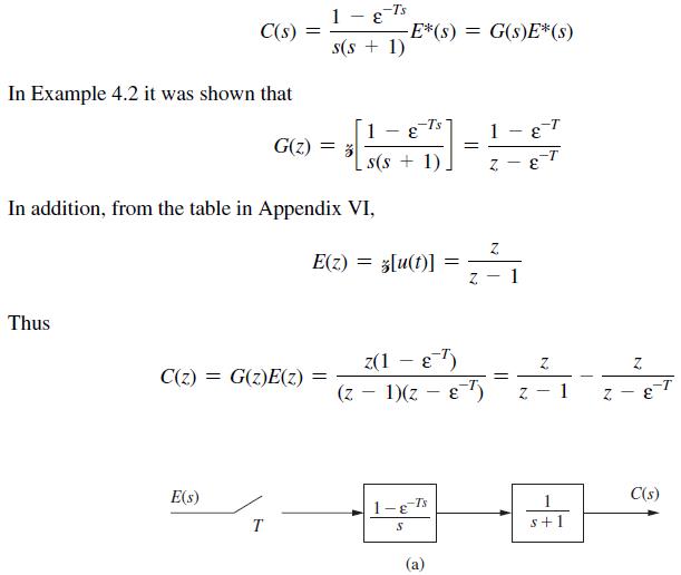
(a) Give the definition of the starred transform.(b) Give the definition of the z-transform.(c) For a function e(t) , derive a relationship between its starred transform E*(s) and its z-transform E(z) .
A signal e(t) is sampled by the ideal sampler as specified by .(a) List the conditions under which e(t) can be completely recovered from e*(t) , that is, the conditions under which no loss of information by the sampling process occurs.(b) State which of the conditions listed in part (a) can
A system is defined as linear if the principle of superposition applies. Is a sampler/zero-order-hold device linear? Prove your answer.
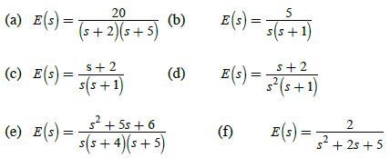
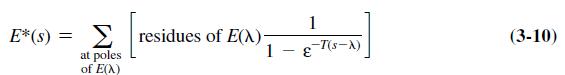
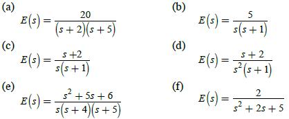
Use the residue method of (3-10) to find the starred transform of the following functions.Equation 3-10 (a) E(s) = (c) E(s) = (e) E(s) = 20 (s+2)(s+5) s+2 s(s+1) s + 5s +6 s(s+4) (s+5) (b) (d) 5 E(5) = s(s+1) E(s) = (f) 5+2 s (s+1) 2 E(S) = 3 +25+5
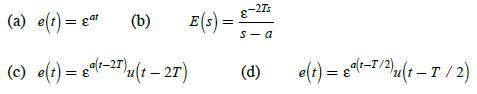
Find E*(s) for each of the following functions. Express E*(s) in closed form. (a) e(t) = gat (c) e(t) = g(1-27)u(1-27) (b) E(s) = -2Ts s-a (d) e(t) = 8(t-1/2)u(t-T / 2)
For e(t) = ε−3t .(a) Express E*(s) as a series.(b) Express E*(s) in closed form.(c) Express E*(s) as a series which is different from that in part (a).
Express the starred transform of e(t − kT) u(t − kT), k an integer, in terms of E*(s) , the starred transform of e(t) . Base your derivation on (3-3).Equation 3-3 E*(s) = E(s) * AT(S)
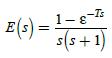
Find E*(s) for E (s) 1-8-7s s(s+1)
(a) Find E*(s) , for T = 0.1 s , for the two functions below. Explain why the two transforms are equal, first from a time-function approach, and then from a pole–zero approach.(i) e1(t) = cos(4πt)(ii) e2 (t) = cos(16πt)(b) Give a third time function that has the same E*(s) .
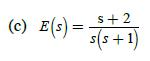
Compare the pole–zero locations of E*(s) in the s-plane with those of E(s) , for the functions given in Problem 3.4-1(c).Problem 3.4-1(c). (c) E(s) = s+2 s(s+1)
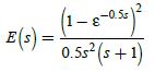
Find E*(s) , with T = 0.5 s , for E(s) = (1-8-0.5) 0.5s (s+1)
Suppose that(a) Find e(kT) for all k.(b) Can e(t) be found? Justify your answer.(c) Sketch two different continuous-time functions that satisfy part (a).(d) Write the equations for the two functions in part (c). * (s) = [e(t)]* = = 1. E*
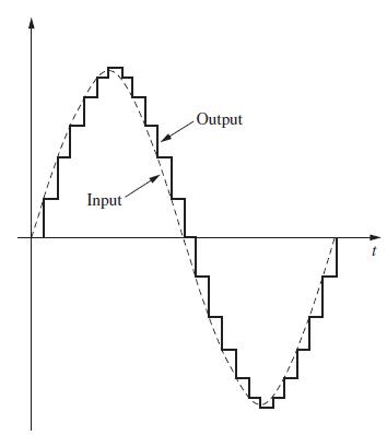
Suppose that the signalis applied to an ideal sampler and zero-order hold.(a) Show that the amplitude of the time function out of the zero-order hold is a function of the phase angle θ by sketching this time function.(b) Show that the component of the signal out of the data hold, at the
(a) A sinusoid with a frequency of 2 Hz is applied to a sampler/zero-order hold combination. The sampling rate is 10 Hz. List all the frequencies present in the output that are less than 50 Hz.(b) Repeat part (a) if the input sinusoid has a frequency of 8 Hz.(c) The results of parts (a) and
Given the signal e(t) = 3sin 4t + 2sin7t.(a) List all frequencies less than ω = 50 rad/s that are present in e(t) .(b) The signal e(t) is sampled at the frequency ωs = 22 rad/s . List all frequencies present in e*(t) that are less than ω = 50 rad/s .(c) The signal e ∗ (t) is applied to a
A signal e(t) = 4sin7t is applied to a sampler/zero-order-hold device, with ω = 4 rad/s .(a) What is the frequency component in the output that has the largest amplitude?(b) Find the amplitude and phase of that component.(c) Sketch the input signal and the component of part (b) versus
It is well known that the addition of phase lag to a closed-loop system is destabilizing. A sampler/data-hold device adds phase lag to a system, as described in Section 3.7. A certain analog control system has a bandwidth of 10 Hz. By this statement we mean that the system (approximately) will
A sinusoid is applied to a sampler/zero-order-hold device, with a distorted sine wave appearing at the output, as shown in Fig. 3-15.(a) With the sinusoid of unity amplitude and frequency 2 Hz, and with fs = 12 Hz , find the amplitude and phase of the component in the output at f1 = 2 Hz
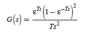
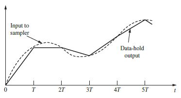
A polygonal data hold is a device that reconstructs the sampled signal by the straight-line approximation shown in Fig. P3.7-8. Show that the transfer function of this data hold isIs this data hold physically realizable? 2 (1 8~ ) Ts G(s)=
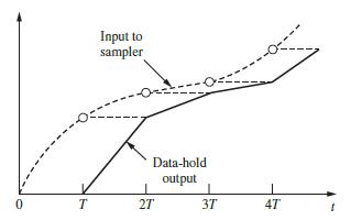
A data hold is to be constructed that reconstructs the sampled signal by the straight-line approximation shown in Fig. P3.7-9. Note that this device is a polygonal data hold with a delay of T seconds. Derive the transfer function for this data hold. Is this data hold physically realizable? 0 T
Plot the ratio of the frequency responses (in decibels) and phase versus for the data holds of Problems 3.7-8 and 3.7-9. Note the effect on phase of making the data hold realizable.Problems 3.7-8A polygonal data hold is a device that reconstructs the sampled signal by the straight-line
Derive the transfer function of the fractional-order hold.
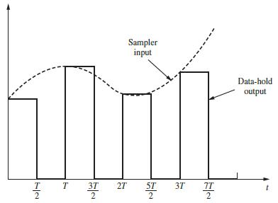
Shown in Fig. P3.7-12 is the output of a data hold that clamps the output to the input for the first half of the sampling period, and returns the output to a value of zero for the last half of the sampling period.(a) Find the transfer function of this data hold.(b) Plot the frequency response of
(a) Show that a pole of E(s) in the left half-plane transforms into a pole of E(z) inside the unit circle.(b) Show that a pole of E(s) on the imaginary axis transforms into a pole of E(z) on the unit circle.(c) Show that a pole of E(s) in the right half-plane transforms into a pole of E(z) outside
Let T = 0.05 s and(a) Without calculating E(z), find its poles.(b) Give the rule that you used in part (a). (c) Verify the results of part (a) by calculating E(z).(d) Compare the zero of E(z) with that of E(s) .(e) The poles of E(z) are determined by those of E(s) . Does an equivalent rule
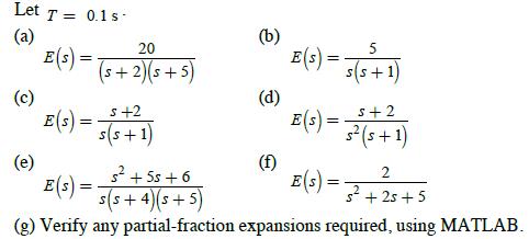
Find the z-transform of the following functions, using z-transform tables. Compare the pole-zero locations of E(z) in the z-plane with those of E(s) and E * (s) in the s-plane. Let T = 0.1s- (a) (c) (e) E(s) = 20 (s+2)(s+5) s+2 E(s) = s(s+1) E(s) = s +55+6 s(s+4) (s+5) (g) Verify any
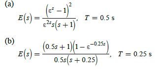
Find the z-transforms of the following functions: (a) (b) E(s) = = E(s) = -1) es(s+1) T = 0.5 s (0.55+1)(1-8-0.25) 0.5s(s+ 0.25) T = 0.25 s
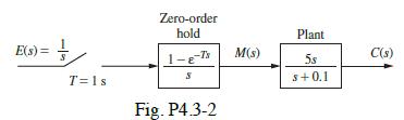
(a) Find the system response at the sampling instants to a unit step input for the system of Fig. P4.3-2. Plot c(nT) versus time.(b) Verify your results of (a) by determining the input to the plant, m(t) , and then calculating c(t) by continuous-time techniques.(c) Find the steady-state gain
(a) Find the conditions on a transfer function G(z) such that its dc gain is zero. Prove your result.(b) Forfind the conditions of Gp (s) such that the de gain of G(z) is zero. Prove your result.(c) Normally, a pole at the origin in the s-plane transforms into a pole at z = 1 in the z-plane. The
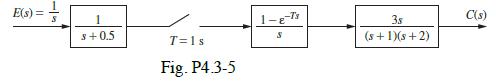
Find the system response at the sampling instants to a unit-step input for the system of Fig. P4.3-5. E(s) = -=-/ 1 3+0.5 T=1s Fig. P4.3-5 1-g-7's S 38 (s + 1)(s+2) C(s)
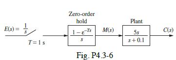
(a) Find the output c(kT) for the system of Fig. P4.3-6, for e(t) equal to a unit-step function.(b) What is the effect on c(kT) of the sampler and data hold in the upper path? Why?(c) Sketch the unit-step response c(t) of the system of Fig. P4.3-6. This sketch can be made without mathematically
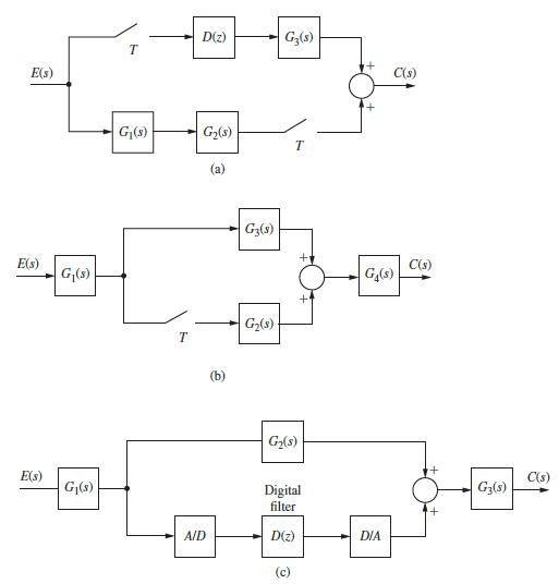
(a) Express each C(s) and C(z) as functions of the input for the systems of Fig. P4.3-7.(b) List those transfer functions in Fig. P4.3-7 that contain the transfer function of a data hold. E(s) E(s) E(s) G(s) G(s) T G(s) T D(z) G(s) (a) A/D (b) G3(8) G(8) G3(s) T G(s) Digital filter D(z) (c) C(s)
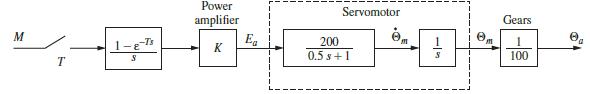
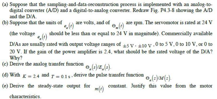
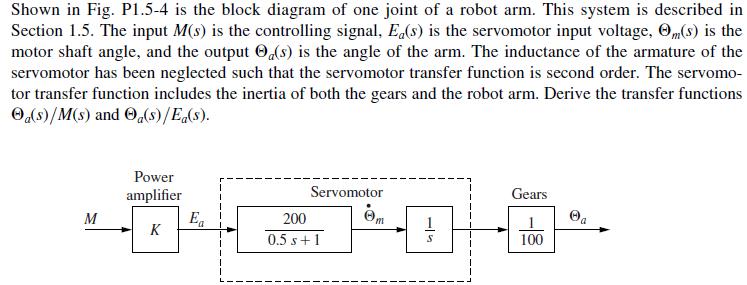
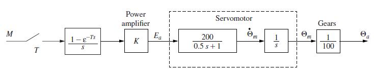
Shown in Fig. P4.3-8 is the block diagram of one joint of a robot arm. This system is described in Problem 1.5-4. The signal M(s) is the sampler input, Ea (s) is the servomotor input voltage, Θm(s) is the motor shaft angle, and the output Θa (s) is the angle of the arm.Problem 1.5-4 M T -Ts 1-a S
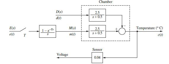
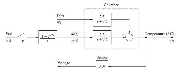
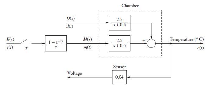
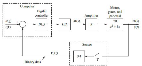
Fig. P4.3-9 illustrates a thermal stress chamber. This system is described in Problem 1.6-1. The system output c(t) is the chamber temperature in degrees Celsius, and the control-voltage input m(t) operates a valve on a steam line. The sensor is based on a thermistor, which is a temperature
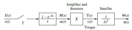
Given in Fig. P4.3-10 is the block diagram of a rigid-body satellite. The control signal is the voltage e(t) . The zero-order hold output m(t) is converted into a torqueτ(t) by an amplifier and the thrusters. The system output is the attitude angleθ(t) of the satellite. E(s) e(t) T 1-8-7's S
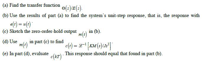
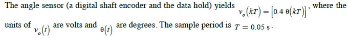
The antenna positioning system described in Section 1.5 and Problem 1.5-1 is depicted in Fig. P4.3-11. In this problem we consider the yaw angle control system, where θ(t) is the yaw angle.(a) Find the transfer function Θ(z)/E(z).(b) The yaw angle is initially zero. The input voltage e(t) is
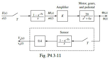
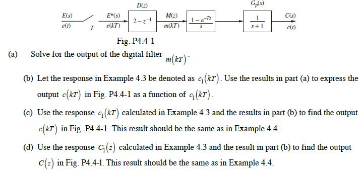
Example 4.3 calculates the step response of the system in Fig. 4-2. Example 4.4 calculates the step response of the same system preceded by a digital filter with the transfer function D(z) = (2 − z−1). This system is shown in Fig. P4.4-1.Example 4.3Given the system shown in Fig. 4-2, with input
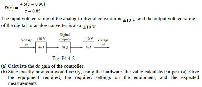
Consider the hardware depicted in Fig. P4.4-2. The transfer function of the digital controller implemented in the computer is given by D(2) = 4.5(z - 0.90) z - 0.85 The input voltage rating of the analog-to-digital converter is +10 V and the output voltage rating of the digital-to-analog converter
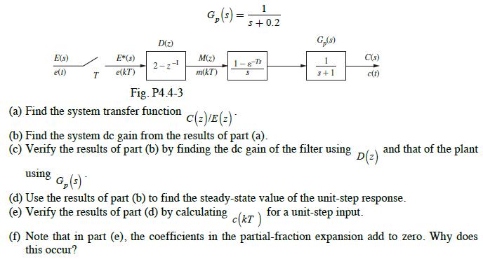
For the system of Fig. P4.4-3, the filter solves the difference equation m(k) = 0.9m(k −1)+ 0.2e(k)The sampling rate is 1 Hz and the plant transfer function is given by E(s) e(t) T using E*(s) e(KT) D(z) 2-z-1 Fig. P4.4-3 (a) Find the system transfer function G (s) = = M(z) m(kT) 1 s+ 0.2 1-g-Ts
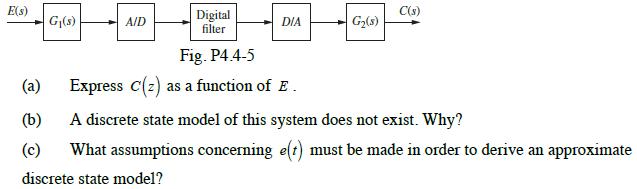
Consider the system of Fig. P4.4-5. The filter transfer function is D(z). E(s) G(s) A/D Digital filter DIA Fig. P4.4-5 Express c(z) as a function of E G(s) C(s) (a) (b) A discrete state model of this system does not exist. Why? (c) What assumptions concerning e(t) must be made in order to derive an
Find the modified z-transform of the following functions: (a) (c) (e) E(s) = 20 (s+2)(s+5) s+2 E(s) = s(s+1) E(s) = s +55+6 s(s+4) (s+5) (b) (d) (f) 5 E(s) = s(s+1) E(s) = E(s) = s+2 s (s+1) 2 s + 25 +5
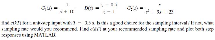
For Problem 4.4-6, assume that the total computational delay in D(z) plus the plant delay totals 3.4T seconds. Repeat the problem under these new conditions.Problem 4.4-6Consider again the system of Fig. P4.4-5. Add a sampler for E(s) at the input. Given G(s) 1 s + 10 D(z) = z - 0.5 z-1 G(s) = S S
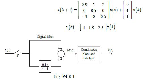
Find a discrete-state-variable representation for the system shown in Fig. P4.8-1. A discrete-state-variable description of the continuous-time system is given by E(s) T Digital filter 0.1z z-1 0.9 1 2 (k+ 1) = 0 0 0.9 0 (k)+ -1 0 0.5 ++ y (k)= [1 1.5 2.3 M(z) Fig. P4.8-1 Continuous plant and data
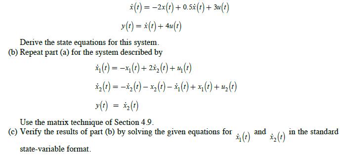
(a) The model of a continuous-time system with algebraic loops is given as x(t)=2x(t) + 0.5x(t) + 3u(t) y(t) = x(t) + 4u(t) Derive the state equations for this system. (b) Repeat part (a) for the system described by xi(t) =xi(t) + 2x(t) + x(t) x(t)=x (t) x (1)- x (t) + x(t) + u(t) y(t) = x(t) Use
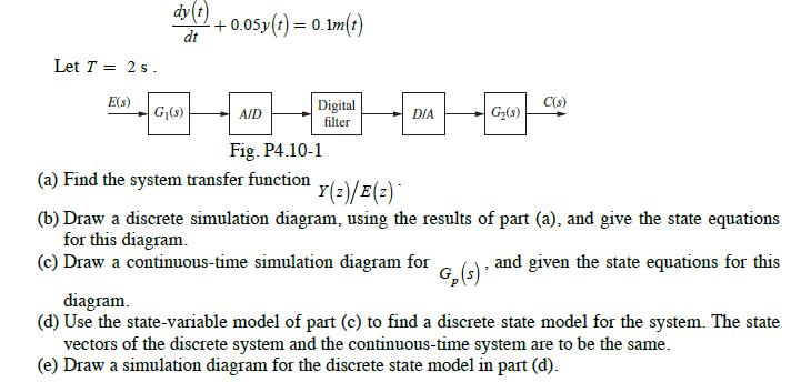
Consider the system of Fig. P4.10-1. The plant is described by the first-order differential equation Let T = 2 s. E(s) dy(t) + 0,05y (t) = 0.1m(t) dt G(s) A/D Digital filter DIA G(s) G (s) C(s) Fig. P4.10-1 (a) Find the system transfer function Y(z)/E(z)* (b) Draw a discrete simulation diagram,
Consider the robot arm system of Fig. P4.3-8. Let T = 0.1 s .(a) Find the system transfer function Θa (z) M(z).(b) Draw a discrete simulation diagram, using the results of part (a), and give the state equations for this diagram.(c) Draw a continuous-time simulation diagram for
Consider the thermal stress chamber depicted in Fig. P4.3-9. Let T = 0.6 s . Ignore the disturbance input d(t) for this problem.(a) Find the system transfer function C(z) E(z) .(b) Draw a discrete simulation diagram, using the results of part (a), and give the state equations for this
Repeat Problem 4.10-4 for the satellite system of Fig. P4.3-10, with T = 1 s . In part (a), the required transfer function is Θ(z) E(z).Problem 4.10-4Consider the thermal stress chamber depicted in Fig. P4.3-9. Let T = 0.6 s. Ignore the disturbance input d(t) for this problem.(a) Find the system
Repeat Problem 4.10-4 for the antenna system of Fig. P4.3-11, with T = 0.05 s . In part (a), the required transfer function is Θ(z) E(z).Problem 4.10-4Consider the thermal stress chamber depicted in Fig. P4.3-9. Let T = 0.6 s. Ignore the disturbance input d(t) for this problem.(a) Find the system
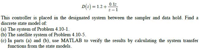
Consider a proportional-integral (PI) digital controller with the transfer function D(z) = 1.2 + 0.1z 2-1 This controller is placed in the designated system between the sampler and data hold. Find a discrete state model of: (a) The system of Problem 4.10-1. (b) The satellite system of Problem
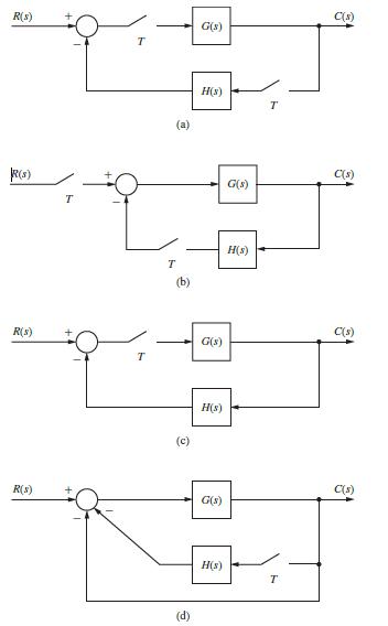
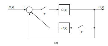
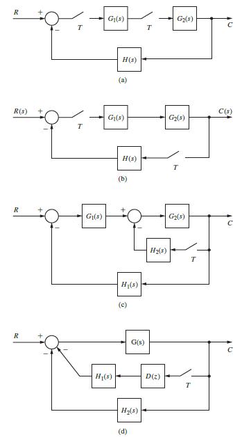
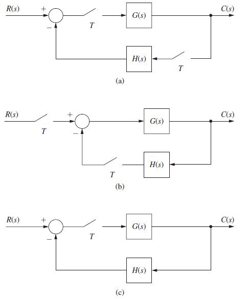
For each of the systems of Fig. P5.3-1, express Error! Objects cannot be created from editing field codes. as a function of the input and the transfer functions shown. R(s) R(8) R(s) R(s) T T T (a) T O (d) G(s) H(s) G(s) H(s) G(s) H(s) K T G(s) H(s) T C(s) C(s) C(s) C(s)
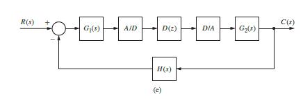
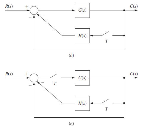
For each of the systems of Fig. P5.3-2, express C (z) as a function of the input and the transfer functions shown. R R(s) R R T T -G(s) G(s) H(s) H(s) (a) G(s) H(s) (b) H(s) 6 G(s) H(8) (d) -G(s) H(s) D(z) G(8) G(s) T T U C(s) C
(a) Derive the transfer function C(z) R(z) for the system of Fig. P5.3-1(b).(b) Derive the transfer function C(z) R(z) for the system of Fig. P5.3-1(c).(c) Even though the two systems are different, the transfer functions are equal. Explain why this is true.
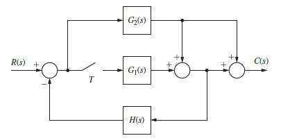
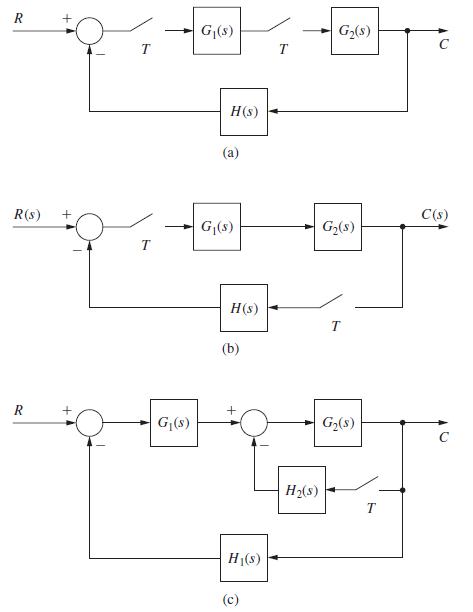
Consider the system of Fig. P5.3-4.(a) Calculate the system output C(z) for the signal fromG2 (s) disconnected from the middlesumming junction.(b) Calculate the system output C(z) for the signal from G2(s) disconnected from the lastsumming junction.(c) Calculate the system output C(z) for the
For the system of Fig. P5.3-1(a), suppose that the sampler in the forward path samples at t = 0, T, 2T, …, and the sampler in the feedback path samples at t = T 2, 3T 2, 5T 2 , . . . . (a) Find the system transfer function C(z) R(z).(b) Suppose that both samplers operate at t = T / 2, 3T / 2, 5T
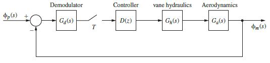
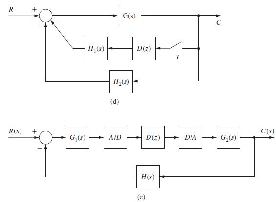
The system of Fig. P5.3-6 contains a digital filter with the transfer function D(z). Express φm(z) as a function of the input. The roll-axis control system of the Pershing missile is of this configuration [2]. op (s) Demodulator Ga(s) T Controller D(z) vane hydraulics Gh(s) Aerodynamics Ga(s)
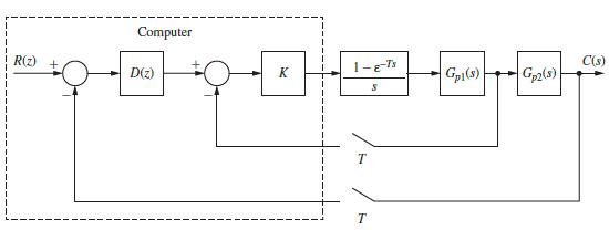
Consider the two-loop system of Fig. P5.3-7. The gain K is used to give the inner loop certain specified characteristics. Then the controller D(z) is designed to compensate the entire system. The input R(z) is generated within the computer, and thus does not exist as a continuous signal. Solve for
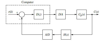
The system of Fig. P5.3-8 is the same as that of Example 5.1, except that the sampler has been moved to the feedback path. This may occur for two reasons: (1) the sensor output is in sampled form and (2) the input function is more conveniently generated in the computer.(a) Calculate both C (s) and
For Fig. P5.3-1, list, for each system, all transfer functions that contain the transfer function of azero-order hold.Fig. P5.3-1 R(s) R(s) R(s) + T T T T (a) (b) G(s) H(s) G(s) H(s) G(s) H(s) T C(s) C(s) C(s)
For Fig. P5.3-2, list, for each system, all transfer functions that contain the transfer function of azero-order hold. R + R(s) + R + T T G(s) G(s) H(s) G(s) H(s) (b) + H(s) (c) T H(s) G(s) G(s) T G(s) T C(s)
In the system of Fig. P5.3-11, the ideal time delay represents the time required to complete the computations in the computer.(a) Derive the output function C(z) for this system.(b) Suppose that the ideal delay is associated with the sensor rather than the computer, and the positions of H(s) and
Consider the satellite control system of Fig. P5.3-14. The units of the attitude angle θ(t) is degrees, and the range is 0 to 360° . The sensor gain is Hk = 0.02 .(a) Suppose that the input ranges for available A/D s are 0 to 5 V, 0 to 10 V, 0 to 20 V, ±5 V ,±10 V , and ±20 V . Which range
Consider the antenna control system of Fig. P5.3-15. The units of the antenna angle θ(t) is degrees, and the range is ±45° .(a) The input signalr (k) is generated in the computer. Find the required values ofr(k) to command the satellite attitude angle θ(t) to be 30° and to be −30° .(b) Let
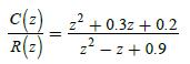
Given a closed-loop system described by the transfer function(a) Express c(k) as a function of r(k), as a single difference equation.(b) Find a set of state equations for this system.(c) Calculate the transfer function from the results of part (b), to verify these results.(d) Verify the results in
For the system of Fig. P5.3-1(a), let T = 0.1 s and(a) Calculate G(z) and H(z) .(b) Draw simulation diagrams for G(z) and H(z) , and interconnect these diagrams to form the control system of Fig. P5.3-1(a).(c) Write the discrete state equations for part (b).(d) Find the system characteristic
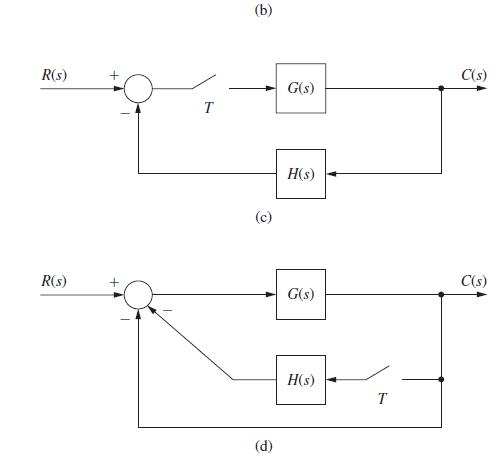
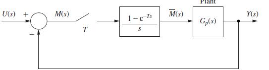
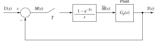
Let T = 0.1 s for the system of Fig. P5.4-4. Derive a set of discrete state equations for the close dloopsystem, for the plant described by each of the differential equations. U(s) + M(s) T 1-8-7's S M(s) Plant Gp(s) Y(s)
Suppose that the plant in Fig. P5.4-4 has the discrete state modelDerive the state model for the closed-loop system, in terms of A, B, C, and D. 1 (k+ 1) = Ax(k) + Bm(k) y (k) = Cx(k) + Dm(k)
Find a discrete state variable model of the closed-loop system shown in Fig. P5.4-4 if the discretestate model of the plant is given by:Fig. P5.4-4 (a) x(k+1)= 0.7x(k)+0.3m (k) y (k) = 0.2x(k) + 0.5m(k) (b) x (x + 1) = 1 (-09 25 X (4) + | 001 m(4) 1.3 0.05 y (k)= [1.2 - 0.7]x (k) 0.5 0 0 (c)
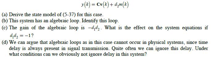
Suppose that, for the system of Fig. 5.4-5, equation (5-34) isFig. 5.4-5 y(k) = Cv (k) + dm (k) (a) Derive the state model of (5-37) for this case. (b) This system has an algebraic loop. Identify this loop. (c) The gain of the algebraic loop is -dd. What is the effect on the system equations if dd
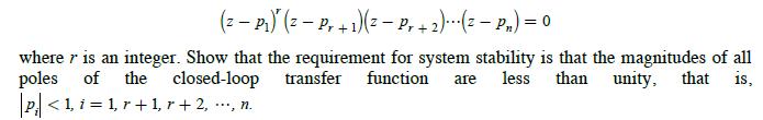
Assume that for the system of Fig. 7-1, the system closed-loop transfer-function pole p1 is repeatedsuch that the system characteristic equation is given byFig. 7-1 (z P) (2 Pr + 1)( Pr + 2)(2 Pn) = 0 where is an integer. Show that the requirement for system stability is that the magnitudes of
Showing 900 - 1000
of 1058
1
2
3
4
5
6
7
8
9
10
11
Step by Step Answers
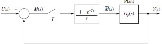
![U(s) T= 0.1 s FIGURE 11-2 Servomotor system. 1 0 2= [8] P(2) = Q = 1--Ts S 1 s(s+ 1) Y(s)](https://dsd5zvtm8ll6.cloudfront.net/images/question_images/1705/5/7/9/82565a9153154fb91705579825191.jpg)
![x(k + 1) y(k) = = 1 0 [1 0.095163 0.904837 0]x (k) x(k) + 0.0048374 0.095163 u(k) (9-1)](https://dsd5zvtm8ll6.cloudfront.net/images/question_images/1705/5/7/9/86765a9155b7149a1705579867383.jpg)

![G(z.) N N 1 [s (s + 1)] = 0.00484Z+0.00468 z1.905z + 0.905](https://dsd5zvtm8ll6.cloudfront.net/images/question_images/1705/5/8/2/25865a91eb2912911705582258072.jpg)

![K = [00 01][B AB.. A B A B a (A) (9-25)](https://dsd5zvtm8ll6.cloudfront.net/images/question_images/1705/5/8/3/96365a9255b6771e1705583962774.jpg)
![x(k+ 1) A B]=[Gc q(k+ 1). GC - BK x(k) BK ][ N(6)] AGC BK (9-56)](https://dsd5zvtm8ll6.cloudfront.net/images/question_images/1705/5/8/4/08665a925d63e5341705584085637.jpg)
![G(z.) = N Z 1 [s (s + 1)] = 0.00484Z+0.00468 z1.905z + 0.905](https://dsd5zvtm8ll6.cloudfront.net/images/question_images/1705/5/8/4/20265a9264aea0de1705584202729.jpg)


![B]=[GCA x(k+ q(k+ 1). -BK A - GCA x(k) BKq(k) (9-74)](https://dsd5zvtm8ll6.cloudfront.net/images/question_images/1705/6/4/0/49765aa023163fc01705640496295.jpg)
![x(k + 1) = Suppose that the output is given by 1 0.0952 0.00484 0.9048] 0.0952|u(k) x(k) + y(k) = [0 1]x(k)](https://dsd5zvtm8ll6.cloudfront.net/images/question_images/1705/6/4/0/63665aa02bc37dd61705640635156.jpg)
![0.0048374 0.095163 Then the gain matrix is, from (9-25), K = [0 1] [B AB] = -95.082 105.082 0.0138934](https://dsd5zvtm8ll6.cloudfront.net/images/question_images/1705/6/4/0/77465aa0346198d91705640773013.jpg)
![x(k+ 1) : - 0 = x(k) + y(k) [10]x(k) = [0.125 25 Ju(k) 0.25](https://dsd5zvtm8ll6.cloudfront.net/images/question_images/1705/6/4/1/03165aa0447db13c1705641030598.jpg)