New Semester Started Get 50% OFF Study Help! --h --m --s Claim Now

Question Answers

Textbooks

Find textbooks, questions and answers

Oops, something went wrong!

Change your search query and then try again

Result Not Found

Books FREE
Study Help
Tutors
AI Study Planner NEW
Sell Books

Search
Sign In
Register

study help
computer science
digital control system analysis and design

Digital Control System Analysis And Design 4th Edition Charles Phillips, H. Nagle, Aranya Chakrabortty - Solutions

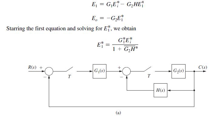
The system of Example 7.1 and Fig. 7-3 has two samplers. The system characteristic equation is derived in Example 7.1 asShow that the same characteristic equation is obtained by opening the system at the second sampler.Example 7.1Consider the system of Example 5.2, which is repeated in Fig. 7-3(a).
(a) The unit-step response of a discrete system is the system response c(k) with the input r(k) = 1 for k ≥ 0 . Show that if the discrete system is stable, the unit-step response, c(k), approaches a constant as k → ∞. [Let T (z) be the closed-loop system transfer function. Assume that the
Consider a sampled-data system with T = 0.5 s and the characteristic equation given by(a) Find the terms in the system natural response.(b) A discrete LTI system is stable, unstable, or marginally stable. Identify the type of stability forthis system.(c) The natural response of this system contains
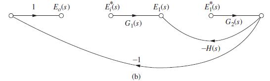
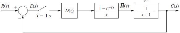
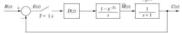
Consider the system of Fig. P7.2-5 with T = 1 s . Let the digital controller be a variable gain K such that D(z) = K . Hence m(kT) = Ke(kT).(a) Write the closed-loop system characteristic equation.(b) Determine the range of K for which the system is stable.(c) Suppose that K is set to the lower
Consider the system of Fig. P7.2-5, and let the digital controller be a variable gain K such that D(z) = K. Hence m(kT) = Ke(kT).(a) Write the closed-loop system characteristic equation as a function of the sample period T.(b) Determine the ranges of K 7 0 for stability for the sample periods T =
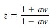
Consider the general bilinear transformationwhere a is real and nonzero.(a) Show that this function transforms the stability boundary of the z-plane into the imaginary axis in the w-plane.(b) Find the relationship of frequency in the s-plane to frequency in the w-plane.(c) Find the stable region
Given below are the characteristic equations of certain discrete systems.(a) Use the Jury test to determine the stability of each of the systems.(b) List the natural-response terms for each of the systems.(c) For those systems in part (a) that are found to be either unstable or marginally
Consider the system of Fig. P7.2-5 with T = 1 s. Let the digital controller be a variable gain K such that D(z) = K. Hence m(kT) = Ke(kT).(a) Write the closed-loop system characteristic equation.(b) Use the Routh–Hurwitz criterion to determine the range of K for stability.(c) Check the results
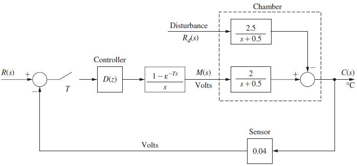
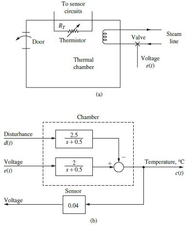
Consider the temperature control system of Fig. P7.5-3. This system is described in Problem 1.6-1. For this problem, ignore the disturbance input, let T = 0.6 s, and let the digital controller be a variable gain K such that D(z) = K. Hence m(kT) = Ke(kT), where e(t) is the input to the sampler. It
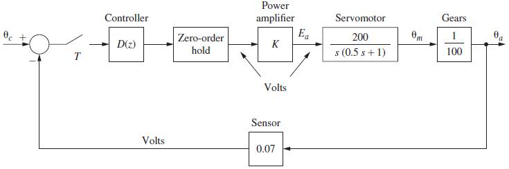
Consider the robot arm joint control system of Fig. P7.5-4. This system is described in Problem 1.5-4. For this problem, T = 0.1 s and D(z) = 1. It was shown in Problem 6-7 that(a) Write the closed-loop system characteristic equation.(b) Use the Routh–Hurwitz criterion to determine the range
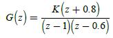
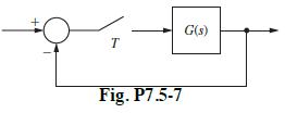
For the system of Fig. P7.5-7, T = 2 s and(a) Determine the range of K for stability using the Routh–Hurwitz criterion.(b) Determine the range of K for stability using the Jury test.(c) Show that the upper limit of K for stability in part (a) yields a marginally stable system.(d) Show that
Given the pulse transfer function G(z) of a plant. For w = 2 rad/s, G (EJWT) is equal to the
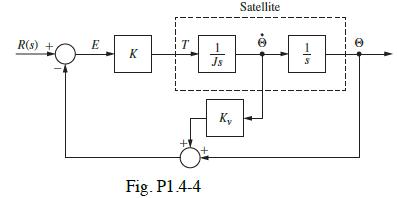
(a) Find the transfer function Θ(s) / Θi (s) for the antenna pointing system of Problem 1.5-1(b). This transfer function yields the angle θ(t) in degrees.(b) Modify the transfer function in part (a) such that use of the modified transfer function yields θ(t) in radians.(c) Verify the
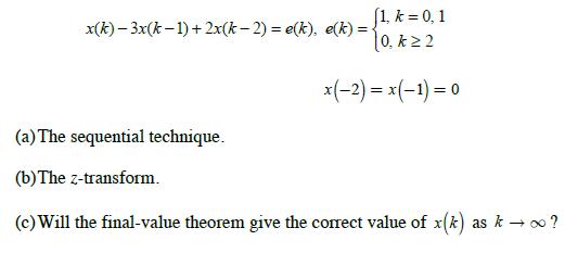
From Table 2-3, *[cos akT] = z(z - cos aT) z - 2z cos aT +1 2
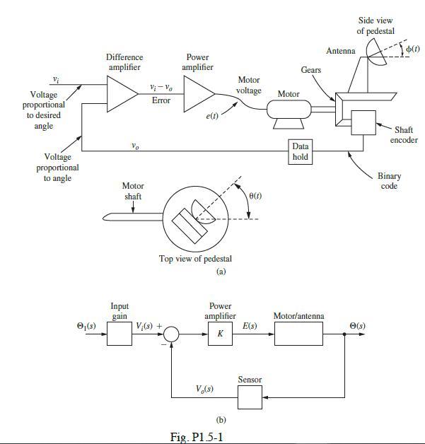
Solve the given difference equation for x(k) using: x(k)-3x(k-1)+2x(k-2)= e(k), e(k) = (1, k = 0, 1 0, k2 x(-2) = x(-1) = 0 (a) The sequential technique. (b) The Z-transform. (c) Will the final-value theorem give the correct value of x(k) as k o?
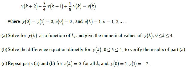
Given the difference equation y(k+ 2) / v(k + 1) + v(k) = e(k) where y(0) = y(1) = 0, e(0) = 0, and e(k) = 1, k = 1, 2,... . (a) Solve for y(k) as a function of k, and give the numerical values of y(k), 0k 4. (b) Solve the difference equation directly for y(k), 0k 4, to verify the results of
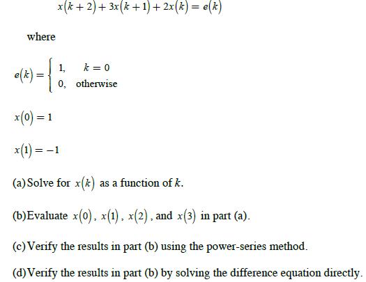
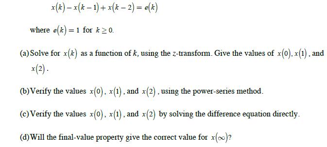
Given the difference equation where e(k)= x(k+ 2) + 3x (k+1) + 2x(k)= e(k) 1, k=0 0, otherwise x(0) = 1 x(1) = -1 (a) Solve for x(x) as a function of k. (b)Evaluate x(0), x(1), x(2), and x(3) in part (a). (c) Verify the results in part (b) using the power-series method. (d) Verify the results in
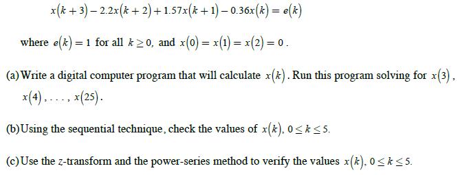
Given the difference equation x(k+ 3) - 2.2x(k+ 2) +1.57x(k+1) 0.36x(k) = e(k) where e(k) = 1 for all k 0, and x(0) = x(1) = x(2) = 0 . (a) Write a digital computer program that will calculate x(k). Run this program solving for x(3), x(4).... x(25). (b) Using the sequential technique, check the
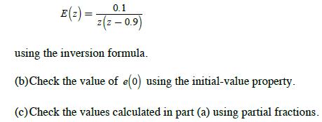
(a) Find e(0) , e(1) , and e(10) for E (2) = 0.1 z(z - 0.9) using the inversion formula. (b)Check the value of e(0) using the initial-value property. (c) Check the values calculated in part (a) using partial fractions.
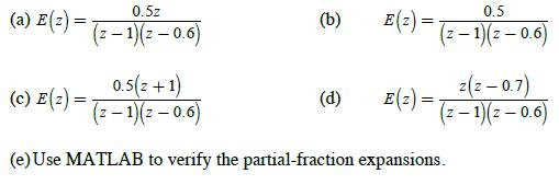
Find the inverse z-transform of each E(z) below by the four methods given in the text. Compare the values of e(z) , for k = 0, 1, 2, and 3, obtained by the four methods. (a) E(z) = 0.5z (2-1)(z-0.6) (c) E () = (b) E (2) = 0.5(z+1) (2-1)(z-0.6) (e) Use MATLAB to verify the partial-fraction
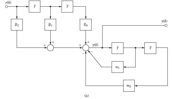
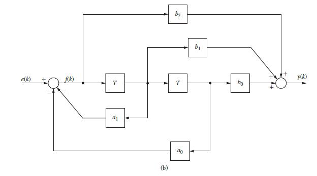
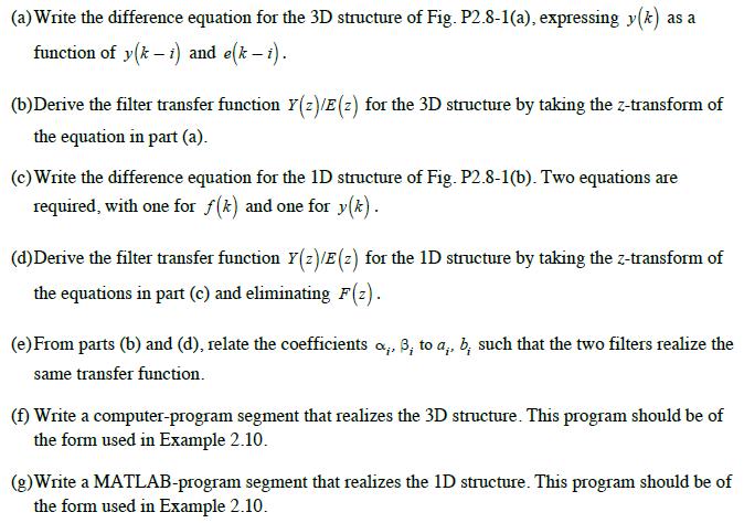
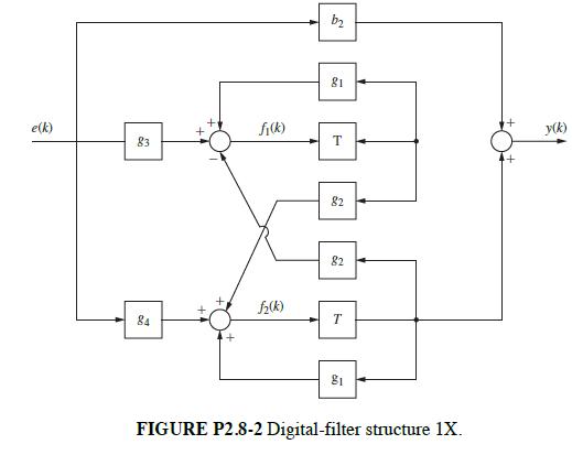
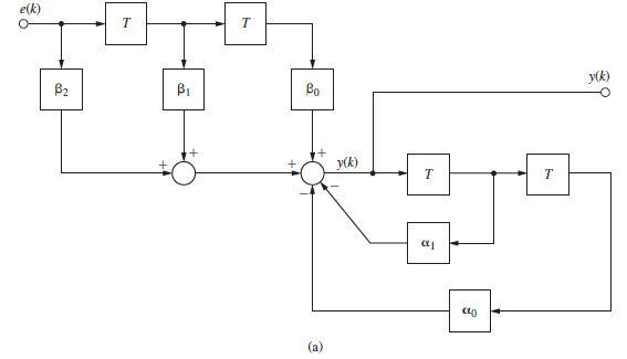
Given in Fig. P2.8-1 are two digital-filter structures, or realizations, for second-order filters.Example 2.10It is desired to find m(k) for the equation B T B T Bo (a) y(k) T 7 3 (x1 CLO T y(k)
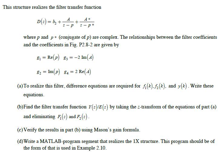
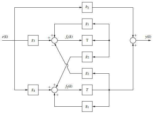
Shown in Fig. P2.8-2 is the second-order digital-filter structure 1X. e(k) 83 84 fi(k) f(k) b 81 T 82 82 T 81 FIGURE P2.8-2 Digital-filter structure 1X. y(k)
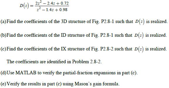
Given the second-order digital-filter transfer functionFigure p2.8-2Figure p2. 8-1 2z-2.4z+0.72 z - 1.4z +0.98 (a) Find the coefficients of the 3D structure of Fig. P2.8-1 such that D(z) is realized. (b) Find the coefficients of the ID structure of Fig. P2.8-1 such that D(z) is realized. (c) Find
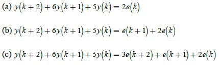
Find two different state-variable formulations that model the system whose difference equation is given by: (a) y(k+ 2) + 6y(k+1) + 5y (k)= 2e(k) (b) y(k + 2) + 6y(k+1) + 5y(k) = e(k+1) + 2e(k) (c) y(k + 2) + 6y (k + 1) + Sy(k) = 3e(k+ 2) + e(k + 1) + 2e(k)
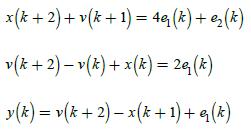
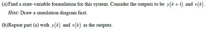
Find a state-variable formulation for the system described by the coupled second-order difference equations given. The system output is y(k) , and e1(k) and e2 (k) are the system inputs. y(k) = v(k + 2) x(k + 1) + q (k) (y) bz = (y) x + (y)-(z+y) (y) + (y) b = (1+y) + (x + y)x
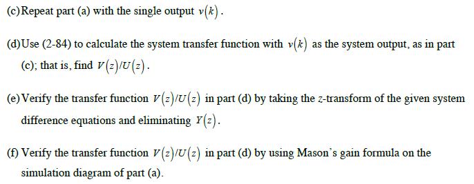
Consider the system described by(a) Find the transfer function Y(z)/U(z).(b) Using any similarity transformation, find a different state model for this system.(c) Find the transfer function of the system from the transformed state equations.(d) Verify that A given and Aw derived in
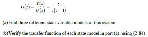
Consider a system with the transfer functionEquation 2-84 Y(z) G() = 2(3) = 2 (2-1) U (a) Find three different state-variable models of this system. (b) Verify the transfer function of each state model in part (a), using (2-84).
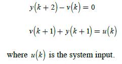
Consider a system described by the coupled difference equationEquation 2-84 y (k+ 2) - v (k)= 0 v(k + 1) + y (k + 1) = u(k) where u(k) is the system input.
Section 2.9 gives some standard forms for state equations (simulation diagrams for the control canonical and observer canonical forms). The MATLAB statementgenerates a standard set of state equations for the transfer function whose numerator coefficients are given in the vector num and denominator
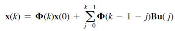
The system described by the equations(a) Use (2-89) to solve for x(k), k ≥0.(b) Find the output y(z) .(c) Show that Φ(k) in (a) satisfies the property Φ(0) = I.(d) Show that the solution in part (a) satisfies the given initial conditions.(e) Use an iterative solution of the state
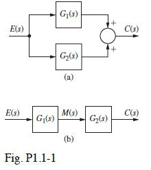
(a) Show that the transfer function of two systems in parallel, as shown in Fig. P1.1-l(a), is equal to the sum of the transfer functions.(b) Show that the transfer function of two systems in series (cascade), as shown in Fig. Pl.1-l(b), is equal to the product of the transfer functions. E(s) E(s)
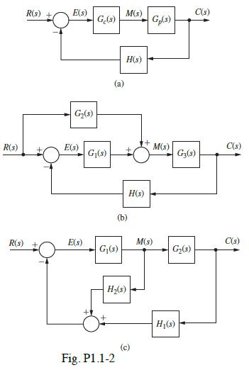
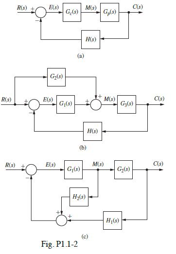
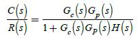
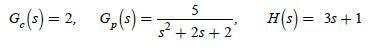
By writing algebraic equations and eliminating variables, calculate the transfer function C(s) R(s) for the system of:(a) Figure P1.1-2(a).(b) Figure P1.1-2(b).(c) Figure P1.1-2(c). R(s) + L R(s) R(s) + E(s) G(8) E(s) E(s) Ge(s) G(s) (a) M(s) G(s) Fig. P1.1-2 H(s) (b) H(s) H(s) (c) Gp(s) M(s)
Use Mason’s gain formula of Appendix II to verify the results of Problem 1.1-2 for the system of:(a) Figure P1.1-2(a).(b) Figure P1.1-2(b).(c) Figure P1.1-2(c). R(s) R(s) R(s) E(s) G(s) E(s) Ge(s) E(s) @ G(s) M(s) G(s) Fig. P1.1-2 H(s) (b) H(s) H(s) Gp(s) (c) M(s) M(s) G(8) H(s) C(s) G3(s) C(s)
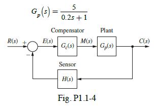
A feedback control system is illustrated in Fig. P1.1-4. The plant transfer function is given by(a) Write the differential equation of the plant. This equation relates c(t) and m(t) .(b) Modify the equation of part (a) to yield the system differential equation; this equation relates c(t) and r(t).
Repeat Problem 1.1-4 with the transfer functionsProblem 1.1-4A feedback control system is illustrated in Fig. P1.1-4. The plant transfer function is given by(a) Write the differential equation of the plant. This equation relates c(t) and m(t) .(b) Modify the equation of part (a) to yield the system
Repeat Problem 1.1-4 with the transfer functionsProblem 1.1-4A feedback control system is illustrated in Fig. P1.1-4. The plant transfer function is given by(a) Write the differential equation of the plant. This equation relates c(t) and m(t) .(b) Modify the equation of part (a) to yield the system
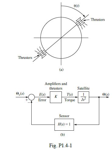
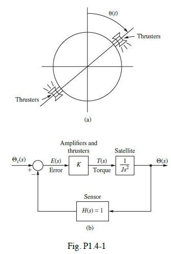
The satellite of Section 1.4 is connected in the closed-loop control system shown in Fig. P1.4-1.The torque is directly proportional to the error signal. Thrusters (s) (a) Amplifiers and thrusters K E(s) Error Sensor H(s) = 1 0(1) T(s) Torque Js Fig. P1.4-1 Satellite Thrusters. e(s)
(a) In the system of Problem 7, J = 0.4 and K = 14.4, in appropriate units. The attitude of the satellite is initially at 0°. At t = 0, the attitude is commanded to 20°; that is, a 20° step is applied at t = 0. Find the response θ(t).(b) Repeat part (a), with the initial conditions θ(0) = 10°
The input to the satellite system of Fig. P1.4-1 is a step function θc (t) = 5u(t) in degrees. As a result, the satellite angle θ(t) varies sinusoidally at a frequency of 10 cycles per minute. Find the amplifier gain K and the moment of inertia J for the system, assuming that the units of time in
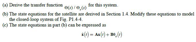
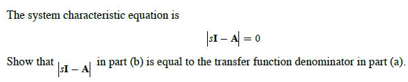
The satellite control system of Fig. P1.4-1 is not usable, since the response to any excitation includes an undamped sinusoid. The usual compensation for this system involves measuring the angular velocity dθ(t) dt . The feedback signal is then a linear sum of the position signal θ(t) and the
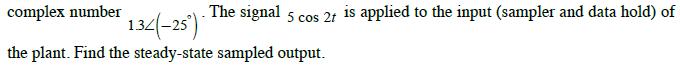
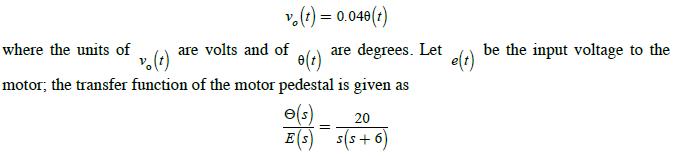
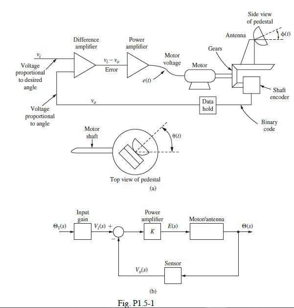
The antenna positioning system described in Section 1.5 is shown in Fig. P1.5–1. In this problem we consider the yaw angle control system, whereθ(t) is the yaw angle. Suppose that the gain of the power amplifier is 10 V/V, and that the gear ratio and the angle sensor (the shaft encoder and the
The state-variable model of a servomotor is given in Section 1.5. Expand these state equations to model the antenna pointing system of Problem 1.5-1(b).Problem 1.5-1(b)The system block diagram is given in Fig. P1.5-1(b), with the angle signals shown in degrees and the voltages in volts. Add the
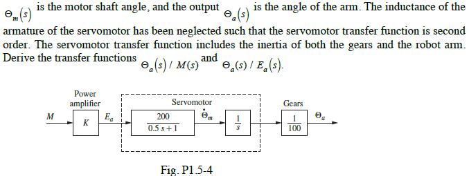
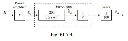
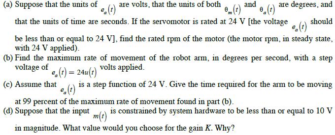
Shown in Fig. P1.5-4 is the block diagram of one joint of a robot arm. This system is described in Section 1.5. The input M(s) is the controlling signal, Ea (s) is the servomotor input voltage, is the motor shaft angle, and the output is the angle of the arm. The inductance of the e(s) m(s)
Consider the robot arm depicted in Fig. P1.5-4.Fig. P1.5-4. M Power amplifier K Ea Servomotor 200 0.5 s +1 Fig. P1.5-4 S I Gears 100 a
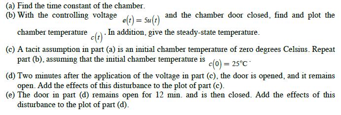
A thermal test chamber is illustrated in Fig. P1.6-1(a). This chamber, which is a large room, is used to test large devices under various thermal stresses. The chamber is heated with steam, which is controlled by an electrically activated valve. The temperature of the chamber is measured by a
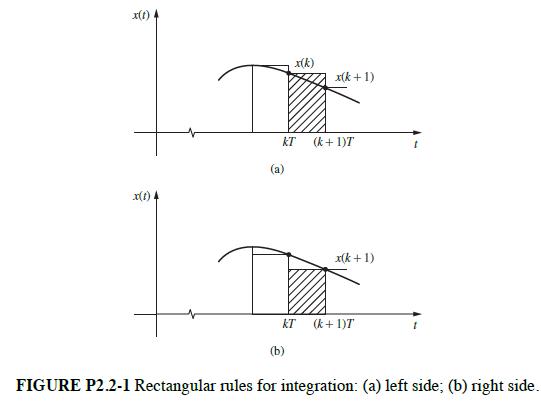
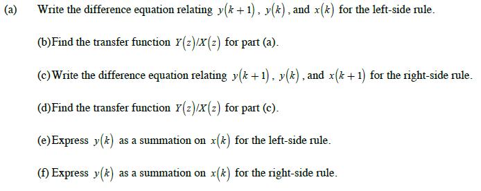
The rectangular rules for numerical integration are illustrated in Fig. P2.2-1. The left-side rule is depicted in Fig. P2.2-1(a), and the right-side rule is depicted in Fig. P2.2-1(b). The integral of x(t)is approximated by the sum of the rectangular areas shown for each rule. Let y(kT) be the
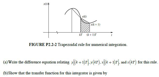
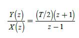
The trapezoidal rule (modified Euler method) for numerical integration approximates the integral of a function x(t) by summing trapezoid areas as shown in Fig. P2.2-2. Let y(t) be the integral of x(t) . x(1)4 x(k) x(k+1) KT (k+ 1)T FIGURE P2.2-2 Trapezoidal rule for numerical integration. (a) Write
Find the z-transform of the number sequence generated by sampling the time function e(t) = t every T seconds, beginning at t = 0 . Can you express this transform in closed form?
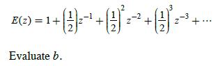
(a) Write, as a series, the z-transform of the number sequence generated by sampling the time function e(t) = ε−t every T seconds, beginning at t = 0 . Can you express this transform in closed form?(b) Evaluate the coefficients in the series of part (a) for the case that T = 0.05 s .(c) The
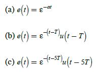
Find the z-transforms of the number sequences generated by sampling the following time functions every T seconds, beginning at t = 0 . Express these transforms in closed form. (a) e(t) = -at 8 (b) e(t) = (-u(t-T) (c) e(t) = 8 (-SI)u(t-5T)
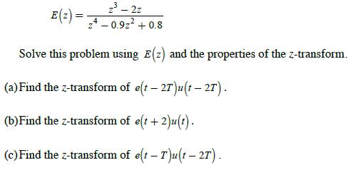
A function e(t) is sampled, and the resultant sequence has the z-transform z - 2z E (2)=4 0.92 +0.8 Solve this problem using E(z) and the properties of the z-transform. (a) Find the z-transform of e(t - 27)u(t-27). (b) Find the z-transform of e(t + 2)u(t). (c) Find the z-transform of e(t -
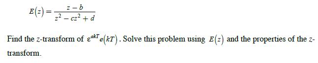
A function e(t) is sampled, and the resultant sequence has the z-transform E (2) = 2-b 2-cz + d Find the z-transform of gate(kr). Solve this problem using E(z) and the properties of the z- transform.
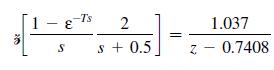
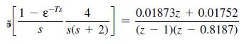
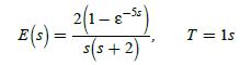
Find the z-transform, in closed form, of the number sequence generated by sampling the time function e(t) every T seconds beginning at t = 0 . The function e(t) is specified by its Laplace transform, E (s) = 2(1-8-) s(s+2) T = 1s
Given the difference equation x(k) - x(k-1) + x(k 2) = e(k) - where e(k)= 1 for k 0. (a) Solve for x(*) as a function of k, using the z-transform. Give the values of x(0), x(1), and x(2). (b) Verify the values x(0), x(1), and x(2), using the power-series method. (c) Verify the values x(0), x(1),
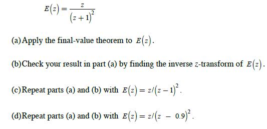
For the number sequence{e(k)}, Z E B () = (= + 1) (a) Apply the final-value theorem to E(z). (b) Check your result in part (a) by finding the inverse z-transform of E(z). (c) Repeat parts (a) and (b) with E(z) = 2/(2-1). (d) Repeat parts (a) and (b) with E(2) = 2/(z - 0.9).
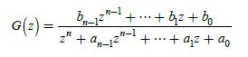
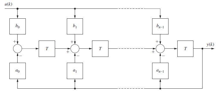
Write the state equations for the observer canonical form of a system, shown in Fig. 2-10, which has the transfer function given in (2-51) and (2-61)Figure 2-10 G(z) = + 2"+an-12"-1 +byz + bo *** + + a+ ao ***
Given the system described by the state equations(a) Calculate the transfer function Y(z)/U(z), using (2-84).(b) Draw a simulation diagram for this system, from the state equations given.(c) Use Mason’s gain formula and the simulation diagram to verify the transfer function found in part
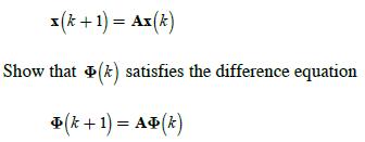
Let Φ(k) be the state transition matrix for the equations x (k+ 1) = Ax(k) Show that (k) satisfies the difference equation (k+ 1) = A (k)

Showing 1000 - 1100 of 1058

1
2
3
4
5
6
7
8
9
10
11

Step by Step Answers

Services

Sitemap
Fun
Definitions
Become Tutor
Used Textbooks
Study Help Categories
Recent Questions
Expert Questions
Campus Wear
Sell Your Books

Company Info

Security
Copyrights
Privacy Policy
Terms & Conditions
SolutionInn Fee
Scholarship
Online Quiz
Give Feedback, Get Rewards

Get In Touch

About Us
Contact Us
Career
Jobs
FAQ
Student Discount
Campus Ambassador

Secure Payment

Download Our App

© 2026 SolutionInn. All Rights Reserved