New Semester Started Get 50% OFF Study Help! --h --m --s Claim Now

Question Answers

Textbooks

Find textbooks, questions and answers

Oops, something went wrong!

Change your search query and then try again

Result Not Found

Books FREE
Study Help
Tutors
AI Study Planner NEW
Sell Books

Search
Sign In
Register

study help
engineering
mechanical vibration analysis

Mechanical Vibrations 6th Edition Singiresu S Rao - Solutions

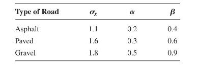
The autocorrelation function of a Gaussian random process representing the unevenness of a road surface is given by\[R_{x}(\tau)=\sigma_{x}^{2} e^{-\alpha|v \tau|} \cos \beta v \tau\]where \(\sigma_{x}^{2}\) is the variance of the random process and \(v\) is the velocity of the vehicle. The values
What are Wiener-Khintchine formulas?
Compute the autocorrelation function corresponding to the ideal white noise spectral density.
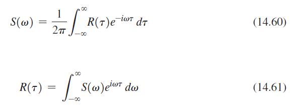
Starting from Eqs. (14.60) and (14.61), derive the relations \[\begin{aligned}& R(\tau)=\int_{0}^{\infty} S(f) \cos 2 \pi f \tau \cdot d f \\& S(f)=4 \int_{0}^{\infty} R(\tau) \cos 2 \pi f \tau \cdot d \tau\end{aligned}\]Equation 14.60 and 14.61:- S(w) = 00 1 2T LR(T)eir R(T)e-iwr dT R(T) =
Write a computer program to find the mean square value of the response of a single-degreeof-freedom system subjected to a random excitation whose power spectral density function is given as \(S_{x}(\omega)\).
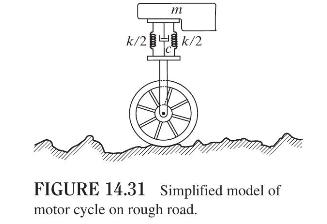
A simplified model of a motorcycle traveling over a rough road is shown in Fig. 14.31. It is assumed that the wheel is rigid, the wheel does not leave the road surface, and the cycle moves at a constant speed \(v\). The cycle has a mass \(m\) and the suspension system has a spring constant \(k\)
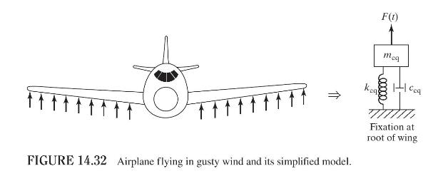
The wing of an airplane flying in gusty wind has been modeled as a spring-mass-damper system, as shown in Fig. 14.32. The undamped and damped natural frequencies of the wing are found to be \(\omega_{1}\) and \(\omega_{2}\), respectively. The mean square value of the displacement of
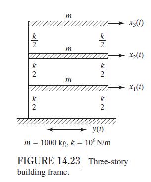
If the building frame shown in Fig. 14.23 has a structural damping coefficient of 0.01 (instead of the modal damping ratio 0.02 ), determine the mean square values of the relative displacements of the various floors.Figure 14.23:- 22 22 *2 m m k 12 X3(1) x2(1) k 2 m x(1) k 2 y(t) m = 1000 kg, k =
The building frame shown in Fig. 14.23 is subjected to a ground acceleration whose power spectral density is given by\[S(\omega)=\frac{1}{4+\omega^{2}}\]Find the mean square values of the relative displacements of the various floors of the building frame. Assume a modal damping ratio of 0.02 in
Using MATLAB, plot the Gaussian probability density function\[f(x)=\frac{1}{\sqrt{2 \pi}} e^{-0.5 x^{2}}\]over \(-7 \leq x \leq 7\).
Plot the Fourier transform of a triangular pulse:\[X(\omega)=\frac{4 A}{a \omega^{2}} \sin ^{2} \frac{\omega a}{2}, \quad-7 \leq \frac{\omega a}{\pi} \leq 7\]
Stroboscopea. produces light pulses intermittentlyb. has high output and is insensitive to temperaturec. frequently used in velocity pickupsd. has high sensitivity and frequency rangee. variable-length cantilever with a mass at its free end
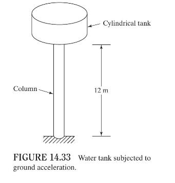
The water tank shown in Fig. 14.33 is supported by a hollow circular steel column. The tank, made of steel, is in the form of a thin-walled pressure vessel and has a capacity of 40,000 litres. Design the column to satisfy the following specifications:(a) The undamped natural frequency of vibration
Using the third-order Runge-Kutta method, solve Problem 11.15.Data From Problem 11.15:-Using the second-order Runge-Kutta method, solve the differential equation \(\ddot{x}+1000 x=0\) with the initial conditions \(x_{0}=5\) and \(\dot{x}_{0}=0\). Use \(\Delta t=0.01\).
Linear acceleration methoda. Assumes that acceleration varies linearly between \(t_{i}\) and \(t_{i}+\theta \Delta t ; \theta \geq 1\)b. Assumes that acceleration varies linearly between \(t_{i}\) and \(t_{i+1}\); can lead to negative dampingc. Based on the solution of equivalent system of
Fill in the Blanks.In a conditionally stable method, the use of \(\Delta t\) larger than \(\Delta t_{\text {cri }}\) makes the method _____________.
The finite difference method requires the use of finite difference approximations ina. governing differential equation onlyb. boundary conditions onlyc. governing differential equation as well as boundary conditions
What is the basic assumption of the Wilson method?
True or False.For a beam with grid points \(-1,1,2,3, \ldots\), the central difference approximation of a simply supported end condition at grid point 1 is given by \(W_{-1}=W_{2}\).
Solve Problem 11.6 by taking the value of \(c\) as 4 .Data From Problem 11.6:-Find the free-vibration response of a viscously damped single-degree-of-freedom system with \(m=k=c=1\), using the central difference method. Assume that \(x_{0}=0, \dot{x}_{0}=1\), and \(\Delta t=0.5
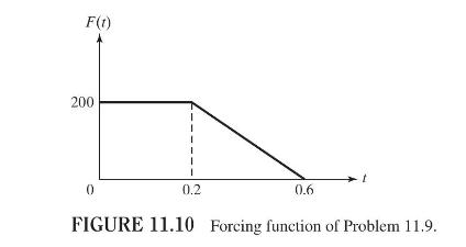
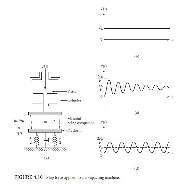
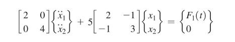
Find the solution of the equation \(4 \ddot{x}+2 \dot{x}+3000 x=F(t)\), where \(F(t)\) is as shown in Fig. 11.10 for the duration \(0 \leq t \leq 1\). Assume that \(x_{0}=\dot{x}_{0}=0\) and \(\Delta t=0.05\). F(1) 200 0 0.2 0.6 FIGURE 11.10 Forcing function of Problem 11.9.
If a bar under longitudinal vibration is fixed at node 1 , the forward difference formula givesa. \(U_{1}=0\)b. \(U_{1}=U_{2}\)c. \(U_{1}=U_{-1}\)
What is a linear acceleration method?
Fill in the Blanks.\(\mathrm{A}(\mathrm{n})\) ________________ formula permits the computation of \(x_{i}\) from known values of \(x_{i-1}\).
True or False.For a beam with grid points \(-1,1,2,3, \ldots\), the central difference approximation of \(\left.\frac{d^{2} W}{d x^{2}}\right|_{1}=0\) yields \(W_{2}-2 W_{1}+W_{-1}=0\).
If a bar under longitudinal vibration is free at node 1 , the forward difference formula givesa. \(U_{1}=0\)b. \(U_{1}=U_{2}\)c. \(U_{1}=U_{-1}\)
What is the difference between explicit and implicit integration methods?
Find the solution of a spring-mass-damper system governed by the equation \(m \ddot{x}+c \dot{x}+k x=F(t)=\delta F . t\) with \(m=c=k=1\) and \(\delta F=1\). Assume the initial values of \(x\) and \(\dot{x}\) to be zero and \(\Delta t=0.5\). Compare the central difference solution with the exact
The central difference approximation of \(d^{4} W / d x^{4}-\beta^{4} W=0\) at grid point \(i\) with step size \(h\) isa. \(W_{i+2}-4 W_{i+1}+\left(6-h^{4} \beta^{4}\right) W_{i}-4 W_{i-1}+W_{i-2}=0\)b. \(W_{i+2}-6 W_{i+1}+\left(6-h^{4} \beta^{4}\right) W_{i}-6 W_{i-1}+W_{i-2}=0\)c. \(W_{i+3}-4
Can we use the numerical integration methods discussed in this chapter to solve nonlinear vibration problems?
Express the following \(n\) th-order differential equation as a system of \(n\) first-order differential equations:\[a_{n} \frac{d^{n} x}{d t^{n}}+a_{n-1} \frac{d^{n-1} x}{d t^{n-1}}+\cdots+a_{1} \frac{d x}{d t}=g(x, t)\]
Houbolt methoda. Assumes that acceleration varies linearly between \(t_{i}\) and \(t_{i}+\theta \Delta t ; \theta \geq 1\)b. Assumes that acceleration varies linearly between \(t_{i}\) and \(t_{i+1}\); can lead to negative dampingc. Based on the solution of equivalent system of first-order
Find the solution of the following equations by using the fourth-order Runge-Kutta method with \(\Delta t=0.1\) :a. \(\dot{x}=x-1.5 e^{-0.5 t} ; x_{0}=1\)b. \(\dot{x}=-t x^{2} ; x_{0}=1\).
Wilson methoda. Assumes that acceleration varies linearly between \(t_{i}\) and \(t_{i}+\theta \Delta t ; \theta \geq 1\)b. Assumes that acceleration varies linearly between \(t_{i}\) and \(t_{i+1}\); can lead to negative dampingc. Based on the solution of equivalent system of first-order
The second-order Runge-Kutta formula is given by\[\vec{X}_{i+1}=\vec{X}_{i}+\frac{1}{2}\left(\vec{K}_{1}+\vec{K}_{2}\right)\]where\[\vec{K}_{1}=h \vec{F}\left(\vec{X}_{i}, t_{i}\right) \quad \text { and } \quad \vec{K}_{2}=h \vec{F}\left(\vec{X}_{i}+\vec{K}_{1}, t_{i}+h\right)\]Using this formula,
Newmark methoda. Assumes that acceleration varies linearly between \(t_{i}\) and \(t_{i}+\theta \Delta t ; \theta \geq 1\)b. Assumes that acceleration varies linearly between \(t_{i}\) and \(t_{i+1}\); can lead to negative dampingc. Based on the solution of equivalent system of first-order
The third-order Runge-Kutta formula is given by\[\vec{X}_{i+1}=\vec{X}_{i}+\frac{1}{6}\left(\vec{K}_{1}+4 \vec{K}_{2}+\vec{K}_{3}\right)\]where\[\begin{gathered}\vec{K}_{1}=h \vec{F}\left(\vec{X}_{i}, t_{i}\right) \\\vec{K}_{2}=h \vec{F}\left(\vec{X}_{i}+\frac{1}{2} \vec{K}_{1}, t_{i}+\frac{1}{2}
Runge-Kutta methoda. Assumes that acceleration varies linearly between \(t_{i}\) and \(t_{i}+\theta \Delta t ; \theta \geq 1\)b. Assumes that acceleration varies linearly between \(t_{i}\) and \(t_{i+1}\); can lead to negative dampingc. Based on the solution of equivalent system of first-order
Using the second-order Runge-Kutta method, solve the differential equation \(\ddot{x}+1000 x=0\) with the initial conditions \(x_{0}=5\) and \(\dot{x}_{0}=0\). Use \(\Delta t=0.01\).
Finite difference methoda. Assumes that acceleration varies linearly between \(t_{i}\) and \(t_{i}+\theta \Delta t ; \theta \geq 1\)b. Assumes that acceleration varies linearly between \(t_{i}\) and \(t_{i+1}\); can lead to negative dampingc. Based on the solution of equivalent system of
Using the fourth-order Runge-Kutta method, solve Problem 11.15.Data From Problem 11.15:-Using the second-order Runge-Kutta method, solve the differential equation \(\ddot{x}+1000 x=0\) with the initial conditions \(x_{0}=5\) and \(\dot{x}_{0}=0\). Use \(\Delta t=0.01\).
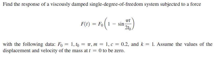
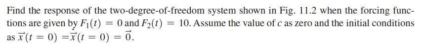
Using the central difference method, find the response of the two-degree-of-freedom system shown in Fig. 11.2 when \(c=2, F_{1}(t)=0, F_{2}(t)=10\).Figure 11.2:- X1(t) -x2(t) F(1) k=2 -F2(t) k = 4 k2=6 00000 m1 1 |m = 21 00000 c = 0 FIGURE 11.2 Two-degree-of-freedom system.
Using the central difference method, find the response of the system shown in Fig. 11.2 when \(F_{1}(t)=10 \sin 5 t\) and \(F_{2}(t)=0\).Figure 11.2:- X1(t) -x2(t) F(1) k=2 -F2(t) k = 4 k2=6 00000 m1 1 |m = 21 00000 c = 0 FIGURE 11.2 Two-degree-of-freedom system.
The equations of motion of a two-degree-of-freedom system are given by \(2 \ddot{x}_{1}+6 x_{1}-2 x_{2}=5\) and \(\ddot{x}_{2}-2 x_{1}+4 x_{2}=20 \sin 5 t\). Assuming the initial conditions as \(x_{1}(0)=\dot{x}_{1}(0)=x_{2}(0)=\dot{x}_{2}(0)=0\), find the response of the system, using the central
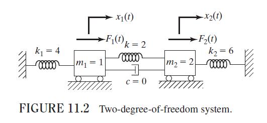
The ends of a beam are elastically restrained by linear and torsional springs, as shown in Fig. 11.11. Using the finite difference method, express the boundary conditions. k W(x) k 00000 Deflected center line of the beam hh ch11- x=0 FIGURE 11.11 Elastically restrained beam. 00000 x=/ k x+
Using the fourth-order Runge-Kutta method, solve Problem 11.20.Data From Problem 11.20:-The equations of motion of a two-degree-of-freedom system are given by \(2 \ddot{x}_{1}+6 x_{1}-2 x_{2}=5\) and \(\ddot{x}_{2}-2 x_{1}+4 x_{2}=20 \sin 5 t\). Assuming the initial conditions as
Find the natural frequencies of a fixed-fixed bar undergoing longitudinal vibration, using three mesh points in the range \(0
Derive the finite difference equations governing the forced longitudinal vibration of a fixedfree uniform bar, using a total of \(n\) mesh points. Find the natural frequencies of the bar, using \(n=4\).
Derive the finite difference equations for the forced vibration of a fixed-fixed uniform shaft under torsion, using a total of \(n\) mesh points.
Find the first three natural frequencies of a uniform fixed-fixed beam.
Derive the finite difference equations for the forced vibration of a cantilever beam subjected to a transverse force \(f(x, t)=f_{0} \cos \omega t\) at the free end.
Derive the finite difference equations for the forced-vibration analysis of a rectangular membrane, using \(m\) and \(n\) mesh points in the \(x\) and \(y\) directions, respectively. Assume the membrane to be fixed along all the edges. Use the central difference formula.
Using Program14.m(fourth-order Runge-Kutta method), solve Problem 11.18 with \(c=1\).Data From Problem 11.18:-Using the central difference method, find the response of the two-degree-of-freedom system shown in Fig. 11.2 when \(c=2, F_{1}(t)=0, F_{2}(t)=10\).Figure 11.2:- X1(t) -x2(t) F(1) k=2
Using Program14 .m (fourth-order Runge-Kutta method), solve Problem 11.19.Data From Problem 11.19:-Using the central difference method, find the response of the system shown in Fig. 11.2 when \(F_{1}(t)=10 \sin 5 t\) and \(F_{2}(t)=0\).Figure 11.2:- X1(t) -x2(t) F(1) k=2 -F2(t) k = 4 k2=6 00000 m1
Using Program15.m (central difference method), solve Problem 11.20.Data From Problem 11.20:-The equations of motion of a two-degree-of-freedom system are given by \(2 \ddot{x}_{1}+6 x_{1}-2 x_{2}=5\) and \(\ddot{x}_{2}-2 x_{1}+4 x_{2}=20 \sin 5 t\). Assuming the initial conditions as
Using Program15.m (central difference method), solve Problem 11.18 with \(c=1\).Data From Problem 11.18:-Using the central difference method, find the response of the two-degree-of-freedom system shown in Fig. 11.2 when \(c=2, F_{1}(t)=0, F_{2}(t)=10\).Figure 11.2:- X1(t) -x2(t) F(1) k=2 -F2(t) k =
Using Program16.m(Houbolt method), solve Problem 11.19.Data From Problem 11.19:-Using the central difference method, find the response of the system shown in Fig. 11.2 when \(F_{1}(t)=10 \sin 5 t\) and \(F_{2}(t)=0\).Figure 11.2:- X1(t) -x2(t) F(1) k=2 -F2(t) k = 4 k2=6 00000 m1 1 |m = 21 00000 c =
Using Program16.m(Houbolt method), solve Problem 11.20.Data From Problem 11.20:-The equations of motion of a two-degree-of-freedom system are given by \(2 \ddot{x}_{1}+6 x_{1}-2 x_{2}=5\) and \(\ddot{x}_{2}-2 x_{1}+4 x_{2}=20 \sin 5 t\). Assuming the initial conditions as
Using the Wilson method with \(\theta=1.4\), solve Problem 11.18.Data From Problem 11.18:-Using the central difference method, find the response of the two-degree-of-freedom system shown in Fig. 11.2 when \(c=2, F_{1}(t)=0, F_{2}(t)=10\).Figure 11.2:- X1(t) -x2(t) F(1) k=2 -F2(t) k = 4 k2=6 00000
Using the Wilson method with \(\theta=1.4\), solve Problem 11.19. 2 618-10-050} 2 4x2 +5 F(t) 3 o
Using the Wilson method with \(\theta=1.4\), solve Problem 11.20.Data From Problem 11.20:-The equations of motion of a two-degree-of-freedom system are given by \(2 \ddot{x}_{1}+6 x_{1}-2 x_{2}=5\) and \(\ddot{x}_{2}-2 x_{1}+4 x_{2}=20 \sin 5 t\). Assuming the initial conditions as
Using the Newmark method with \(\alpha=\frac{1}{6}\) and \(\beta=\frac{1}{2}\), solve Problem 11.18.Data From Problem 11.18:-Using the central difference method, find the response of the two-degree-of-freedom system shown in Fig. 11.2 when \(c=2, F_{1}(t)=0, F_{2}(t)=10\).Figure 11.2:- X1(t) -x2(t)
Using the Newmark method with \(\alpha=\frac{1}{6}\) and \(\beta=\frac{1}{2}\), solve Problem 11.19.Data From Problem 11.19:-Using the central difference method, find the response of the system shown in Fig. 11.2 when \(F_{1}(t)=10 \sin 5 t\) and \(F_{2}(t)=0\).Figure 11.2:- X1(t) -x2(t) F(1) k=2
The equations of motion of a two-degree-of-freedom system are given bywhere \(F_{1}(t)\) denotes a rectangular pulse of magnitude 5 acting over \(0 \leq t \leq 2\). Find the solution of the equations using MATLAB. 2 618-10-050} 2 4x2 +5 F(t) 3 o
Using the Newmark method with \(\alpha=\frac{1}{6}\) and \(\beta=\frac{1}{2}\), solve Problem 11.20.Data From Problem 11.20:-The equations of motion of a two-degree-of-freedom system are given by \(2 \ddot{x}_{1}+6 x_{1}-2 x_{2}=5\) and \(\ddot{x}_{2}-2 x_{1}+4 x_{2}=20 \sin 5 t\). Assuming the
Find the response of a simple pendulum numerically by solving the exact equation:\[\ddot{\theta}+\frac{g}{l} \sin \theta=0\]with \(\frac{g}{l}=0.01\) and plot the response, \(\theta(t)\), for \(0 \leq t \leq 150\). Assume the initial conditions as \(\theta(t=0)=\theta_{0}=1 \mathrm{rad}\) and
Using MATLAB function ode23, solve the differential equation \(5 \ddot{x}+4 \dot{x}+3 x=6 \sin t\) with \(x(0)=\dot{x}(0)=0\).
Find the response of a simple pendulum numerically by solving the linearized equation:\[\ddot{\theta}+\frac{g}{l} \theta=0\]with \(\frac{g}{l}=0.01\) and plot the response, \(\theta(t)\), for \(0 \leq t \leq 150\). Assume the initial conditions as \(\theta(t=0)=\theta_{0}=1 \mathrm{rad}\) and
Find the response of a simple pendulum numerically by solving the nonlinear equation:\[\ddot{\theta}+\frac{g}{l}\left(\theta-\frac{\theta^{3}}{6}\right)=0\]with \(\frac{g}{l}=0.01\) and plot the response, \(\theta(t)\), for \(0 \leq t \leq 150\). Assume the initial conditions as
Write a subroutine wILSON for implementing the Wilson method. Use this program to find the solution of Example 11.7.Data From Example 11.7:-Data From Example 11.3:- Find the response of the system considered in Example 11.3, using the Wilson method with 0 = 1.4.
Write a subroutine NUMARK for implementing the Newmark method. Use this subroutine to find the solution of Example 11.8.Data From Example 11.8:-Data From Example 11.3:- 91 Find the response of the system considered in Example 11.3, using the Newmark method with a = and = .
For a bar element of length \(l\) with two nodes, the shape function corresponding to node 1 is given bya. \(\left(1-\frac{x}{l}\right)\)b. \(\frac{x}{l}\)c. \(\left(1+\frac{x}{l}\right)\)
What is the basic idea behind the finite element method?
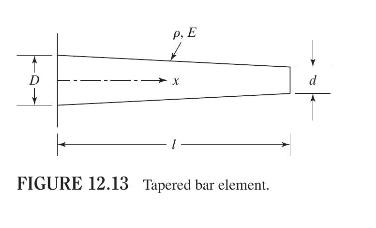
Derive the stiffness matrix of the tapered bar element (which deforms in the axial direction) shown in Fig. 12.13. The diameter of the bar decreases from \(D\) to \(d\) over its length. P. E D X d FIGURE 12.13 Tapered bar element.
True or False.For a bar element of length \(l\) with two nodes, the shape function corresponding to node 2 is given by \(x / l\).
Fill in the Blank.In the finite element method, the solution domain is replaced by several ___________.
The simplest form of mass matrix is known asa. lumped-mass matrixb. consistent-mass matrixc. global mass matrix
What is a shape function?
True or False.The element stiffness matrices are always singular.
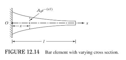
Derive the stiffness matrix of the bar element in longitudinal vibration whose cross-sectional area varies as \(A(x)=A_{0} e^{-(x / l)}\), where \(A_{0}\) is the area at the root (see Fig. 12.14). Age-(x/1) FIGURE 12.14 Bar element with varying cross section.
Fill in the Blank.In the finite element method, the elements are assumed to be interconnected at certain points known as ____________ .
The finite element method isa. an approximate analytical methodb. a numerical methodc. an exact analytical method
What is the role of transformation matrices in the finite element method?
True or False.The element mass matrices are always singular.
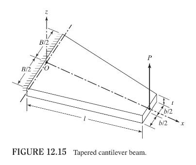
The tapered cantilever beam shown in Fig. 12.15 is used as a spring to carry a load \(P\). Derive the stiffness matrix of the beam using a one-element idealization. Assume \(B=25 \mathrm{~cm}\), \(b=10 \mathrm{~cm}, t=2.5 \mathrm{~cm}, l=2 \mathrm{~m}, E=2.07 \times 10^{11} \mathrm{~N} /
Fill in the Blank.In the finite element method, \(a(n)\) ___________ solution is assumed within each element.
The stiffness matrix of a bar element is given bya. \(\frac{E A}{l}\left[\begin{array}{ll}1 & 1 \\ 1 & 1\end{array}\right]\)b. \(\frac{E A}{l}\left[\begin{array}{rr}1 & -1 \\ -1 & 1\end{array}\right]\)c. \(\frac{E A}{l}\left[\begin{array}{ll}1 & 0 \\ 0 & 1\end{array}\right]\)
What is the basis for the derivation of transformation matrices?
True or False.The system stiffness matrix is always singular unless the boundary conditions are incorporated.
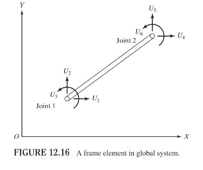
Derive the stiffness and mass matrices of the planar frame element (general beam element) shown in Fig. 12.16 in the global \(X Y\)-coordinate system. Y U U3 U Joint 1 Joint 2 U6 Us UA FIGURE 12.16 A frame element in global system. X
Fill in the Blank.The displacement within a finite element is expressed in terms of _____________ functions.
The consistent mass matrix of a bar element is given bya. \(\frac{ho A l}{6}\left[\begin{array}{ll}2 & 1 \\ 1 & 2\end{array}\right]\)b. \(\frac{ho A l}{6}\left[\begin{array}{rr}2 & -1 \\ -1 & 2\end{array}\right]\)c. \(\frac{ho A l}{6}\left[\begin{array}{ll}1 & 0 \\ 0 & 1\end{array}\right]\)
How are fixed boundary conditions incorporated in the finite element equations?
True or False.The system mass matrix is always singular unless the boundary conditions are incorporated.
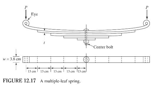
A multiple-leaf spring used in automobiles is shown in Fig. 12.17. It consists of five leaves, each of thickness \(t=0.65 \mathrm{~cm}\) and width \(w=3.8 \mathrm{~cm}\). For the multiple-leaf spring described in Fig. 12.17, derive the assembled stiffness and mass matrices. Consider only one-half
Fill in the Blank.For a thin beam element, __________ degrees of freedom are considered at each node.
The boundary condition corresponding to the free end of a bar in longitudinal vibration is given bya. \(u(0, t)=0\)b. \(\frac{\partial u}{\partial x}(0, t)=0\)c. \(A E \frac{\partial u}{\partial x}(0, t)-u(0, t)=0\)
Fill in the Blank.The lateral vibration of a thin beam is governed by a(n) _________ order partial differential continuous system.
Free enda. Bending moment \(=0\); shear force equals theb. Deflection \(=0\); slope \(=0\)c. Deflection \(=0\); bending moment \(=0\)d. Bending moment \(=0\); shear force \(=0\)
True or False.The Rayleigh-Ritz method assumes that the solution is a series of functions that satisfy the boundary conditions of the problem.

Showing 900 - 1000 of 2655

First
3
4
5
6
7
8
9
10
11
12
13
14
15
16
17
Last

Step by Step Answers

Services

Sitemap
Fun
Definitions
Become Tutor
Used Textbooks
Study Help Categories
Recent Questions
Expert Questions
Campus Wear
Sell Your Books

Company Info

Security
Copyrights
Privacy Policy
Terms & Conditions
SolutionInn Fee
Scholarship
Online Quiz
Give Feedback, Get Rewards

Get In Touch

About Us
Contact Us
Career
Jobs
FAQ
Student Discount
Campus Ambassador

Secure Payment

Download Our App

© 2026 SolutionInn. All Rights Reserved