New Semester Started Get 50% OFF Study Help! --h --m --s Claim Now

Question Answers

Textbooks

Find textbooks, questions and answers

Oops, something went wrong!

Change your search query and then try again

Result Not Found

Books FREE
Study Help
Tutors
AI Study Planner NEW
Sell Books

Search
Sign In
Register

study help
engineering
mechanical vibration analysis

Mechanical Vibration Analysis, Uncertainties, And Control 4th Edition Haym Benaroya, Mark L Nagurka, Seon Mi Han - Solutions

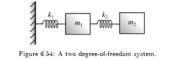
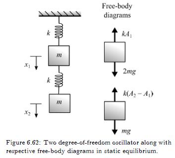
Suppose that for the two degree-of-freedom system of Figure 6.54 we obtain the data: \(f_{1}=4 \mathrm{~Hz}, f_{2}=\) \(10 \mathrm{~Hz}, f_{3}=8 \mathrm{~Hz}\), and \(m_{1}+m_{2}=20 \mathrm{~kg}\). Solve for the system parameters \(k_{1}, k_{2}, m_{1}, m_{2}\). 1 k k www mm m- Figure 6.54: A two
Since liquids have damping characteristics, suggest possible equivalent mechanical models for a sloshing liquid that includes damping.
Suppose a container with interior fluid is in an aircraft. The aircraft leaves on its flight with full tanks and arrives at its destination with almost empty tanks. How could this fact be incorporated in the equivalent mechanical model?
Suppose a container with interior fluid is in a spacecraft in orbit around the Earth. What additional considerations need to be incorporated in the equivalent mechanical model?
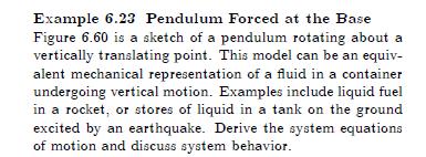
In Example 6.23, solve for \(\theta(t)\) analytically for the case \(g Example 6.23 Pendulum Forced at the Base Figure 6.60 is a sketch of a pendulum rotating about a vertically translating point. This model can be an equiv- alent mechanical representation of a fluid in a container undergoing
Derive Equations 6.154 and 6.155 using Newton's second law of motion. Le+(+9) sin=0. (6.154)
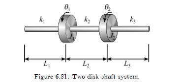
For a two disk torsional system (see Figure 6.81) with its two ends fixed to walls, follow the procedure of Example 6.24 to evaluate the two approximate frequencies of oscillation. Explain the procedure used to guess the respective mode shapes. Check that the approximate fundamental frequency is
How would Rayleigh's quotient need to be altered for an unrestrained system? Apply the method to a general two degree-of-freedom undamped system in unrestrained rectilinear motion.
Derive Equation 7.4,\[\frac{\partial}{\partial x}\left[T(x) \frac{\partial y}{\partial x}\right]+f(x, t)=m(x) \frac{\partial^{2} y}{\partial t^{2}}\]using Newton's second law of motion.
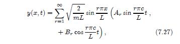
Solve for the string response, Equation 7.27, given the following initial conditions:(a) \(y(x, 0)=0, \dot{y}(x, 0)=g(x)\)(b) \(y(x, 0)=\sin \pi x / L, \dot{y}(x, 0)=0\)(c) \(y(x, 0)=0, \dot{y}(x, 0)=\sin \pi x / L\)(d) \(y(x, 0)=\sin \pi x / L, \dot{y}(x, 0)=\sin \pi x / L\).In all cases, sketch
Derive the expression for the tension required in a simply supported transmission line modeled as a string of length \(l\) and linear density \(ho\), such that its fundamental frequency for transverse vibration is \(f_{1}\). What is the value of the tension where \(l=20\) \(\mathrm{m}, ho=5
A string is stretched between \(x=0\) and \(x=L\) and has a variable density \(ho=ho_{0}+\varepsilon x\), where \(ho_{0}\) and \(\varepsilon\) are constants. The initial displacement is \(f(x)\), and the string is released from rest.(a) If the tension \(T\) is constant, then show that the governing
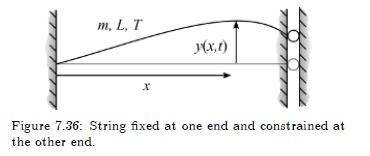
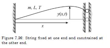
Consider the uniform string with constant mass per unit length \(m\), constant tension \(T\), and length \(L\), shown in Figure 7.36. One end of the string is fixed, and the other end is constrained to move in the vertical direction. Find the frequency equation, the first three natural frequencies,
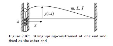
Consider the uniform string with constant mass per unit length \(m\), constant tension \(T\), and length \(L\) shown in Figure 7.37. One end of the string is fixed, and the other end is attached to a spring with stiffness \(k\) that is constrained to move in the vertical direction. Find the
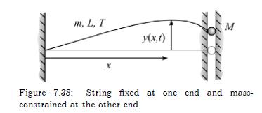
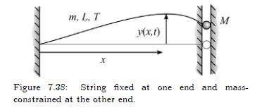
Consider the uniform string with constant mass per unit length \(m\), constant tension \(T\), and length \(L\) shown in Figure 7.38. One end of the string is fixed, and the other end is attached to a mass \(M\) that is constrained to move in the vertical direction. Find the frequency equation, the
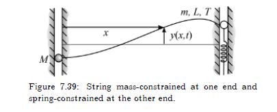
Consider the uniform string with constant mass per unit length \(m\), constant tension \(T\), and length \(L\) shown in Figure 7.39. One end of the string is attached to a mass \(M\) and the other end of the string is constrained by a spring with stiffness \(k\). Both ends are constrained to move
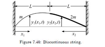
Consider the fixed-fixed uniform string made of two sections shown in Figure 7.40. The left section of the string has a constant mass per unit length \(m\), and the right section of the string has the constant mass per unit length \(2 m\). (a) From a free-body diagram and Newton's second law of
Plot the displacement response of the string in Figure 7.36 at \(x=L\) as a function of time if the initial displacement is \(y(x, 0)=0.05 x / L\) and the initial velocity is zero. m, L, T x y(x,t) 77777 Figure 7.36: String fixed at one end and constrained at the other end.
Plot the displacement response of the string in Figure 7.36 at \(x=L\) if the string is initially horizontal and is subject to the sinusoidal input force at \(x=L, F(t)=F_{0} \sin \omega_{f} t\). Use \(L=1 \mathrm{~m}, T=100 \mathrm{~N}\), \(m=0.2 \mathrm{~kg} / \mathrm{m}, \omega_{f}=10
Plot the displacement response of the string in Figure 7.38 at \(x=L\) as a function of time if the initial displacement is \(y(x, 0)=0.05 x / L\) and the initial velocity is zero. The orthogonality condition for the eigenfunctions must be obtained first. m. L, T M y(x,t) X Figure 7.38: String
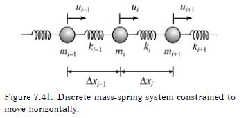
Consider a system consisting of discrete masses connected by springs in series as shown in Figure 7.41. Derive the equation of motion for mass \(m_{i}\) using Newton's second law, arrange the equation in incremental form, take the limit, and derive the differential equation of motion for the
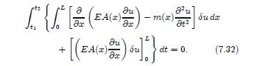
Derive Equation 7.32. [{[(EA)))]de ]}] EA(x)- -m(x). Su dx + [(EA(x)) bu] * } d dt = 0. (7.32)
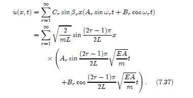
For the uniform fixed-fixed beam in longitudinal vibration shown in Figure 7.42 derive the expressions for the natural frequencies and the mode shapes. Sketch the first three modes. x m, EA L Figure 7.42: Fixed-fixed beam in longitudinal vibration.
For Equation 7.37, solve for the constants \(A_{r}\) and \(B_{r}\) by satisfying the initial conditions. M8 M8 u(x,t) = C, sin 3x(A, sin wrt + B+ cos wrt) 2 (2-1) sin -x mL 2L XA, sin (2-1) EA 2L m (2r 1) EA +B, cos t (7.37) 2L
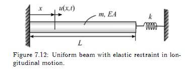
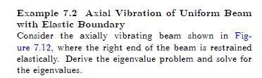
Complete the solution of Example 7.2 for the modes and the complete solution. Example 7.2 Axial Vibration of Uniform Beam with Elastic Boundary Consider the axially vibrating beam shown in Fig- ure 7.12, where the right end of the beam is restrained elastically. Derive the eigenvalue problem and
Consider the free axial motion of a beam with the elastic boundary conditions of Example 7.2, and solve for the first four natural frequencies, modes, and the complete solution, for the following cases:(a) \(k=E A \mathrm{~N} / \mathrm{m}, L=10 \mathrm{~m}\)(b) \(k=10 E A \mathrm{~N} / \mathrm{m},
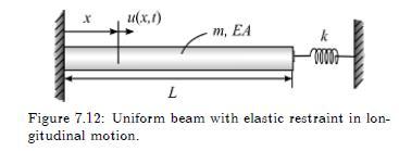
An unrestrained beam lies on a horizontal and smooth surface and at \(t=0\) is forced at one end by \(F(t)\), as shown in Figure 7.43. Derive the general response for any forcing function using the known eigenvalues and eigenfunctions. Then evaluate the specific steady-state response for the
Find the response of a uniform beam clamped at \(x=0\) and free at \(x=L\) subjected to the longitudinal force,\[ f(x, t)=F_{o} \delta[x-(L-\varepsilon)] u(t) \]
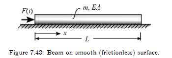
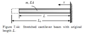
Derive the natural frequencies and mode shapes of the longitudinally vibrating uniform beam of Figure 7.44. Sketch the first three mode shapes. What will change in the analysis if the beam is vertical? m. EA x L Lo Figure 7.44: Stretched cantilever beam with original length L.
A cantilever beam has its free end stretched uniformly so that the original length \(L\) becomes \(L_{0}\), and then it is released at \(t=0\), as shown in Figure 7.44. Begin with the general solution for the axial response of a beam,\[ \begin{aligned} u(x, t)= & \sum_{r=1}^{\infty} \sin
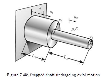
Consider the stepped shaft made of the same material of density \(ho\) and modulus \(E\), shown in Figure 7.45. Determine the characteristic equation for the natural frequencies of the system as it undergoes axial motion. Let \(u_{1}(x, t)\) denote the displacement in the shaft with the fixed end,
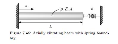
Consider the uniform beam shown in Figure 7.46. Solve for the lowest natural frequency of axial motion of the steel beam given the following parameter values: \(E=210 \mathrm{GN} / \mathrm{m}^{2}, ho=7850 \mathrm{~kg} / \mathrm{m}^{3}, L=1.2\) \(\mathrm{m}, k=100 \mathrm{kN} / \mathrm{m}\), and
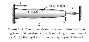
Solve for the first three modes and frequencies of the nonuniform longitudinally vibrating beam of Figure 7.47 beginning with the known equation of motion. The following properties hold:\[ \begin{aligned} E A(x) & =2 E A(1-x / L) \\ \text { and } m(x) & =2 m(1-x / L) \end{aligned}
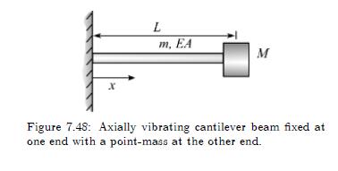
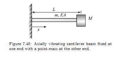
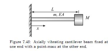
Consider the longitudinally vibrating uniform beam shown in Figure 7.48. One end of the beam is fixed and the other end is free with an attached concentrated mass \(M\). Derive the frequency equation, the first three natural frequencies, and plot the first three mode shapes for axial vibration. Use
Derive the orthogonality condition for the eigenfunctions of the beam shown in Figure 7.48. x L m, EA M Figure 7.48: Axially vibrating cantilever beam fixed at one end with a point-mass at the other end.
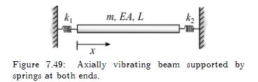
Consider the longitudinally vibrating uniform beam shown in Figure 7.49. The ends of the beam are supported by linear springs with stiffnesses \(k_{1}\) and \(k_{2}\). Derive the frequency equation, the first three natural frequencies, and plot the first three mode shapes for axial vibration. Use
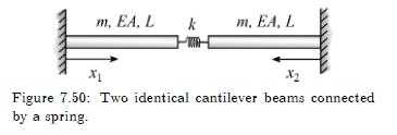
Consider the two identical longitudinally vibrating uniform beams shown in Figure 7.50 connected by a linear spring. Derive the frequency equation, the first three natural frequencies, and plot the first three mode shapes for axial vibration. Use \(k L / E A=0.1\). m, EA, L k m, EA, L x1 X2 Figure
Plot the response of the concentrated mass in Figure 7.48 due to the initial displacement \(u(x, 0)=\) \(0.02 x / L\) and zero initial velocity. x L m, EA M Figure 7.48: Axially vibrating cantilever beam fixed at one end with a point-mass at the other end.
Consider a fixed-fixed uniform torsional beam with length \(L\), torsional rigidity \(G J\), and mass per unit length \(m\). Derive the frequency equation, the first three natural frequencies, and plot the first three mode shapes.
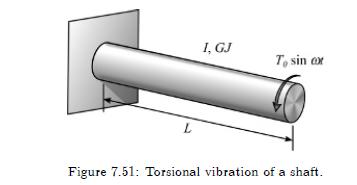
The uniform shaft of Figure 7.51 is subjected to the torque \(T_{0} \sin \omega t\) at its free end. (a) Find the steadystate vibration response by solving the free vibration problem, including the forcing function in a boundary condition. (b) Solve this problem as a forced vibration problem where
Complete the general solution for \(\theta(x, t)\), assuming the arbitrary initial conditions \(\theta(x, 0)\) and \(\dot{\theta}(x, 0)\).
Solve for the frequencies, the modes and the total response \(\theta(x, t)\) of the system for the cases:(a) \(I L=I_{D}\),(b) \(I L=10 I_{D}\),(c) \(I L=I_{D} / 10\).
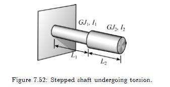
Consider the stepped shaft consisting of two uniform segments of lengths \(L_{1}\) and \(L_{2}\), torsional rigidities \(G J_{1}\) and \(G J_{2}\), and mass moments of inertia per unit length \(I_{1}\) and \(I_{2}\), shown in Figure 7.52. Set up the eigenvalue problem for the torsional vibration of
In the oil drilling industry, a drill-tube is used for well-boring. It is a tube of outer diameter \(D_{o}\) and inner diameter \(D_{i}\) and is made of steel of density \(ho\) and modulus of rigidity \(G\). At the end of the drill-tube there is a drill bit that does the actual drilling. (The bit
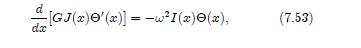
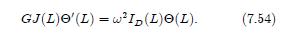
Derive Equations 7.53 and 7.54. [GJ(x)0'(x)] = w1(x)0(x), (7.53) dx
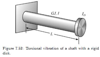
A circular elastic shaft of length \(L\) has one end clamped and a rigid disk attached at the other end, as shown in Figure 7.53. If \(G\) denotes the modulus of rigidity, \(J\) the area polar moment of inertia of the shaft, \(I\) the mass polar moment of inertia of the shaft per unit length, and
Derive the frequency equation, the first three natural frequencies, and plot the first three mode shapes of a clamped-clamped uniform beam undergoing transverse vibration.
Derive the frequency equation, the first three natural frequencies, and plot the first three mode shapes of a clamped-pinned uniform beam undergoing transverse vibration.
Derive the frequency equation, the first three natural frequencies, and plot the first three mode shapes of a clamped-uniform beam with a concentrated mass \(M\) at the free end undergoing transverse oscillation. Use \(M / m L=1\).
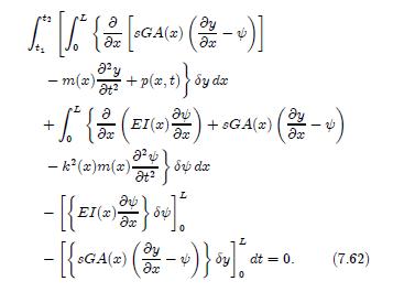
Perform the necessary variations to derive Equation 7.62 . y [8GA(x) (0-4)] -m(x)- + p(x, t) by dx t + EI(x)- : ) + GA(2) (3/2/2-4) -k2(x)m(x)- - t EI(x) L (-)}]* -[{GA(x) ( x dt = 0. (7.62)
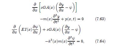
Equations 7.63 and 7.64 are solved using the assumed solutions \(y(x, t)=Y(x) \exp (i \omega t)\) and \(\psi(x, t)=\Psi(x) \exp (i \omega t)\). Find the characteristic equation. a [GA(2) x 2 -m(x). +p(x,t) = 0 (7.63) t 3 (EI (x) 3x)- + GA(x) (x-4) -k(x)m(x)- 0. (7.64) t
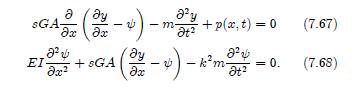
In Equations 7.67 and 7.68, eliminate \(y(x, t)\) and derive the governing equation for \(\psi(x, t)\). What physical motion does this equation govern? SGAx SGA (3) a y t m- +p(x,t) = 0 (7.67) 0-10-(-1)x+2 (7.68)
Derive the Bernoulli-Euler beam equation, Equation 7.74. State all assumptions. a SGA- m- t +p(x,t) = 0 (7.67)
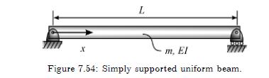
For the simply supported uniform beam of Figure 7.54 undergoing transverse motion, derive the natural frequencies and the natural modes of vibration. Sketch the first three mode shapes. What will change in the analysis if the beam is on an inclined surface? X L m, El Figure 7.54: Simply supported
For the transverse vibration of a simply supported uniform beam, solve for the transient response if the initial conditions are given by\[ y(x, 0)=B\left(\frac{x}{L}-3 \frac{x^{2}}{L^{2}}+2 \frac{x^{3}}{L^{3}}\right) \quad \dot{y}(x, 0)=0 \]
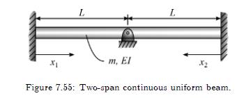
A two-span uniform beam may be used as a simple model of a bridge. For this model, sketched in Figure 7.55 , derive the frequency equation. L L m, El Figure 7.55: Two-span continuous uniform beam.
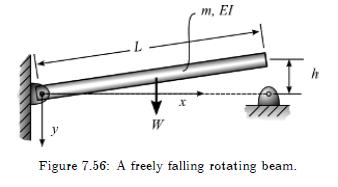
The beam of Figure 7.56 is released and rotates as a rigid body and impacts at an angular speed of \(\Omega\) \(\mathrm{rad} / \mathrm{s}\). Assume that upon impact the beam latches onto the support and there is no rebound and no loss in energy. At impact the beam transfers all of its rotational
Determine the characteristic equation for the transverse vibration of a beam that is pinned at one end and free at the other end.
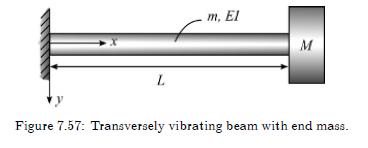
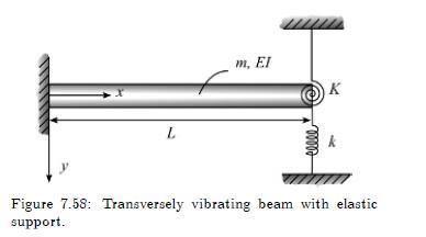
List the boundary conditions for the transversely vibrating beams of Figures 7.57 and 7.58. L m, El M Figure 7.57: Transversely vibrating beam with end mass.
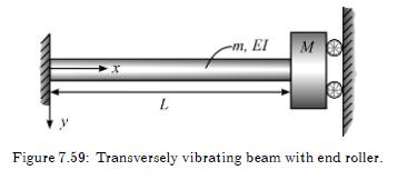
For the transversely vibrating beam of Figure 7.59 , find the modes and the first three natural frequencies of vibration. L -m, El M Figure 7.59: Transversely vibrating beam with end roller.
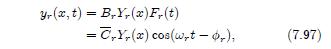
Complete the solution of Equation 7.97 for the initial conditions \(y(x, 0)=d(x)\) and \(\dot{y}(x, 0)=v(x)\). yr(x,t) =BY,(x) Fr(t) =Y,(x) cos(wyt - or), (7.97)
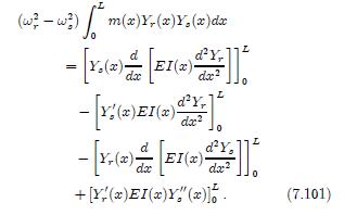
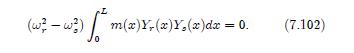
Derive Equation 7.102 beginning with Equation 7.101 . (ww) m(x)Y+(x)Y.(x)dx - [Y.(x) [EI(x) = da -[Y' (2) EI (2) dY, dY, da doc2 [[ d'Y, [Y-(*) [E1(2)]] dx +(x)EI(x)Y" (x)]. (7.101)
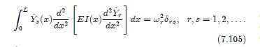
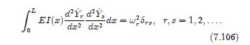
Derive Equation 7.106 starting with Equation 7.105. Y (2) d2 da2 EI(x) = dx dawr, r, 1, 2,.... = (7.105)
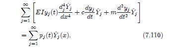
Fill in the steps in the derivation of Equation 7.110. Ely; (t) 5 dx4 =p;(t)(x). +c 1Y + m dt dt (7.110)
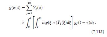
Solve Equation 7.113 for zero initial conditions and for each of the following forcing functions:(a) \(p(x, t)=u(t)\), where \(u(t)\) is the unit step function(b) \(p(x, t)=\sin \Omega t\)(c) \(p(x, t)=e^{-\varphi t}\), for \(t \geq 0\)(d) \(p(x, t)=\sin \Omega t\), for \(0 \leq \Omega \leq \pi /
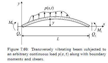
Derive the equation of motion and boundary conditions for a transversely vibrating beam using Hamilton's principle. Assume small deflections. Let \(I_{p}\) equal the mass moment of inertia per unit length of the beam about its neutral axis. Figure 7.60 provides a sketch of the beam along with
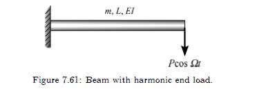
Solve for the response of the cantilever beam sketched in Figure 7.61. m, L, EI Pcos Figure 7.61: Beam with harmonic end load.
In Example 7.7, solve for the case where \(t=\tau_{1} / 4\). Example 7.7 Evaluation of Arbitrary Constants and Vibration-Induced Stresses Continue Example 7.4 by evaluating the arbitrary con- stants A, and o, of Equation 7.92. Also, connect vibra- tion and stress to the fatigue life of structures.
Find the response of a simply supported beam subjected to the external moment at \(x=L\),\[ p(x, t)=M(t) u^{\prime \prime}(x-L) \]
Derive the equation of motion for the transversely vibrating beam with axial force by applying Hamilton's principle.
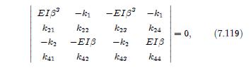
Solve Equation 7.119 by setting the determinant of the coefficients equal to zero, resulting in a polynomial that is solved for the frequencies. Use the following parameter values: \(E=30 \times 10^{6} \mathrm{lb} / \mathrm{in}^{2}\), \(I=10 \times 10^{4} \mathrm{in}^{4}, k_{1}=100 \mathrm{lb} /
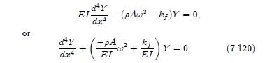
Derive Equation 7.120. or 10 d da-4 - (pAw - k+)Y = 0, dY + -PA w + da4 (+) Y = 0. (7.120)
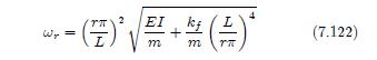
Derive Equation 7.122. Wy = + =(2) + ()* m m (7.122)
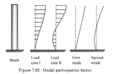
Discuss the modal participation factor for a vibrating beam that is subjected to loads as shown in Figure 7.62. Beam Load Load First Second case I case II mode mode Figure 7.62: Modal participation factor.
Solve the equations of motion using the Laplace transform approach, where \(v(t)\) is the speed and \(F(t)\) is the force:(a) \(\dot{v}+2 v=F(t), v(0)=1, F(t)=0\)(b) \(2 \dot{v}+2 v=F(t), v(0)=0, F(t)=10\)(c) \(\dot{v}+3 v=F(t), v(0)=1, F(t)=2 \sin (3 t)\).
Solve the equations of motion using the Laplace transform approach:(a) \(\ddot{x}+3 \dot{x}+2 x=0, x(0)=1, \dot{x}(0)=0\)(b) \(2 \ddot{x}+5 \dot{x}+3 x=0, x(0)=1, \dot{x}(0)=1\)(c) \(\ddot{x}+2 \dot{x}+2 x=0, x(0)=2, \dot{x}(0)=4\)(d) \(\ddot{x}+2 \dot{x}+x=0, x(0)=1, \dot{x}(0)=-1\)(e)
Solve the equations of motion using the Laplace transform approach:(a) \(\ddot{x}+3 \dot{x}+2 x=u(t), x(0)=1, \dot{x}(0)=0\)(b) \(2 \ddot{x}+5 \dot{x}+3 x=e^{-3 t}, x(0)=1, \dot{x}(0)=1\)(c) \(\ddot{x}+2 \dot{x}+2 x=\cos t, x(0)=2, \dot{x}(0)=4\)(d) \(\ddot{x}+2 \dot{x}+x=e^{-2 t}+\sin 2 t, x(0)=1,
Solve the equations of motion using the Laplace transform approach:(a) \(\ddot{y}+2 \dot{y}+3 y=5 \cos 3 t, y(0)=3, \dot{y}(0)=4\)(b) \(4 \ddot{y}+5 \dot{y}+5 y=4 u(t), y(0)=1, \dot{y}(0)=1\), where \(u(t)\) is the unit step function(c) \(3 \ddot{y}+3 \dot{y}+6 y=3 e^{-t}+2 \cos 3 t, y(0)=2,
For the given transfer functions, find the response of the system due to the unit step input force \(F(t)=\) \(u(t)\) and zero initial conditions:(a) \(X(s) / \mathcal{F}(s)=1 /(s+2)\)(b) \(X(s) / \mathcal{F}(s)=1 /\left(s^{2}+3 s+2\right)\)(c) \(X(s) / \mathcal{F}(s)=(3 s+2) /\left(s^{2}+3
For the given transfer functions, find the response of the system due to the input force \(F(t)=\) \(2 \cos (3 t) u(t)\) and zero initial conditions:(a) \(X(s) / \mathcal{F}(s)=1 /(s+2)\)(b) \(X(s) / \mathcal{F}(s)=1 /\left(s^{2}+3 s+2\right)\)(c) \(X(s) / \mathcal{F}(s)=1 /\left(s^{2}+2
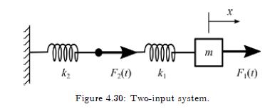
Consider a system subjected to two input forces, as shown in Figure 4.30. Find the transfer functions, \(X(s) / \mathcal{F}_{1}(s)\) and \(X(s) / \mathcal{F}_{2}(s)\). Find the response \(x(t)\) due to \(F_{1}(t)=t\) and \(F_{2}(t)=u(t)\). Use zero initial conditions, and let \(m=1 \mathrm{~kg},
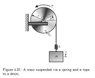
A mass of \(m=50 \mathrm{~kg}\) is suspended by a spring attached to a rope that is wound around a drum with radius \(r=0.4 \mathrm{~m}\) and moment of inertia about the point of rotation \(I_{O}=45 \mathrm{~kg} \mathrm{~m}^{2}\), as shown in Figure 4.31. The spring of stiffness \(k=3 \mathrm{kN} /
Derive Equation 4.19:\[ v(t)=\frac{1}{\omega_{n}^{2}}\left[1-e^{-\zeta \omega_{n} t}\left(\cos \omega_{d} t+\frac{\zeta \omega_{n}}{\omega_{d}} \sin \omega_{d} t\right)\right] \]for \(t \geq 0\).
Assuming \(\zeta
Using the Laplace transform, solve\[ \ddot{y}+2 \dot{y}+y=F(t) \]where\[ F(t)=u(t-1)-2 u(t-2)+u(t-3) \]is in terms of unit step functions, and \(y(0)=0\) and \(\dot{y}(0)=0\).
Find the impulse response function of a system whose equation of motion is given by(a) \(\dot{x}+4 x=f(t)\)(b) \(\ddot{x}+4 x=f(t)\)(c) \(\ddot{x}+5 \dot{x}+4 x=f(t)\)(d) \(\ddot{x}+2 \dot{x}+x=f(t)\)(e) \(\ddot{x}+5 \dot{x}+4 x=5 \dot{f}(t)+4 f(t)\).
Find the impulse response function of a system whose transfer function is given by(a) \(G(s)=1 /(2 s+1)\)(b) \(G(s)=1 /\left(2 s^{2}+3 s+1\right)\)(c) \(G(s)=1 /\left(s^{2}+4 s+4\right)\)(d) \(G(s)=1 /\left(s^{2}+9\right)\)(e) \(G(s)=(5 s+4) /\left(s^{2}+5 s+4\right)\).
Find the response of each of the systems given below to arbitrary inputs, \(f(t)\) :(a) \(\dot{x}+4 x=f(t), f(t)=u(t)\)(b) \(\ddot{x}+4 x=f(t), f(t)=t, t \geq 0\)(c) \(\ddot{x}+5 \dot{x}+4 x=f(t), f(t)=1\) for \(0 \leq t
Find the response of the undamped oscillator \(\ddot{x}+\) \(4 x=F(t) / m\) to each of the following forces per unit mass using the convolution integral:(a) \(F(t) / m=1-e^{-t}, t \geq 0\)(b) \(F(t) / m=\cos 2 t, 0 \leq t \leq \pi\)(c) \(F(t) / m=\cos 2 t+3,0 \leq t \leq \pi\)(d) \(F(t) / m=\cos 2
Find the response of the damped oscillator \(\ddot{x}+\) \(2 \zeta \omega_{n} \dot{x}+\omega_{n}^{2} x=F(t) / m\), with \(\omega_{n}^{2}=4(\mathrm{rad} / \mathrm{s})^{2}\), to the forces per unit mass listed, and solve for the two underdamped cases of \(\zeta=0.1\) and \(\zeta=0.9\) :(a) \(F(t) /
Solve for the damped response beginning with the equation,\(x(t)=\frac{1}{m \omega_{d}} \int_{0}^{t} \sin \omega(t-\tau) \exp \left(-\zeta \omega_{n} \tau\right) \sin \omega_{d} \tau d \tau\).In the same graph, plot the results for the following cases:\[ \omega=1.0,1.5,2.0,2.5,3.0 \mathrm{rad} /
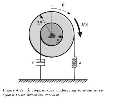
The stepped disk in Figure 4.32 is subject to the moment\[ M(t)=1-e^{-t}, t \geq 0 \]The spring is unstretched when \(\theta=0\). Derive the equation of motion and solve for the response \(\theta(t)\) assuming zero initial conditions and an underdamped system. 2R R eelle M(1) Figure 4.32: A
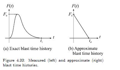
Structures are sometimes subjected to very rapidly applied loads of extremely short duration. These types of loads are called blast or explosive loads. Consider how such a load time history may look. Figure 4.33(a) is a generic blast load. There is a rapid rise time along with an exponential-like
Resolve Problem 19 including damping. Discuss the importance of damping by comparing the two results. Problem 19:Structures are sometimes subjected to very rapidly applied loads of extremely short duration. These types of loads are called blast or explosive loads. Consider how such a load time
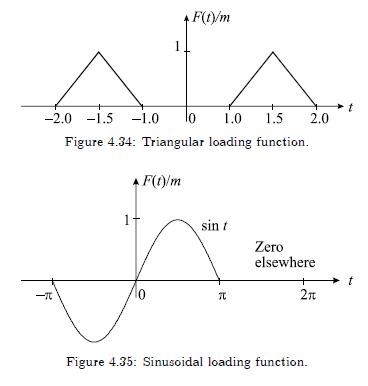
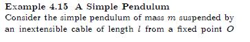
Solve for the response for all time of an underdamped oscillator that is driven by the forcing function shown in (a) Figure 4.34, and (b) Figure 4.35. Use the convolution integral. -2.0 -1.5 -1.0 1 F(t)/m t 1.0 1.5 2.0 Figure 4.34: Triangular loading function. F(t)/m 1 sin t Zero 10 elsewhere
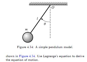
Use Lagrange's equation to derive the equation of motion for the simple pendulum of Example 4.15, except here assume that the mass \(m\) is suspended on a rigid bar that is connected to the support via a torsional spring of stiffness \(K\). Example 4.15 A Simple Pendulum Consider the simple
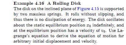
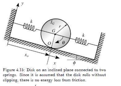
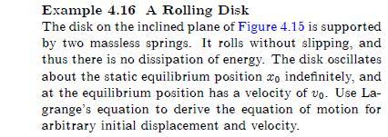
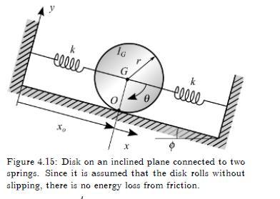
For Example 4.16 derive the equation of motion using \(x\) as the generalized coordinate. Then solve this equation with initial conditions \(x_{0}, v_{0}\) to find\[ x(t)=\frac{v_{0}}{\omega} \sin \omega t-\frac{m g}{2 k} \sin \phi(\cos \omega t-1)+x_{0} \]where \(\omega=\sqrt{4 k / 3 m}\).
Derive the equation of motion of Example 4.16 using Newton's second law of motion. Example 4.16 A Rolling Disk The disk on the inclined plane of Figure 4.15 is supported by two massless springs. It rolls without slipping, and thus there is no dissipation of energy. The disk oscillates about the
For the problem of oscillator control, given by Equation 4.32, consider the specific governing equation\[ \ddot{x}+2 \zeta \omega_{n} \dot{x}+\omega_{n}^{2} x=\frac{A}{m} \cos \omega t+F_{\text {control }}(t) \]where \(\zeta, \omega_{n}\), and \(F_{\text {control }}(t)\) must be determined so
How does randomness of excitation alter the analyst's ability to evaluate structural response?

Showing 200 - 300 of 2655

1
2
3
4
5
6
7
8
9
10
11
12
13
14
15
Last

Step by Step Answers

Services

Sitemap
Fun
Definitions
Become Tutor
Used Textbooks
Study Help Categories
Recent Questions
Expert Questions
Campus Wear
Sell Your Books

Company Info

Security
Copyrights
Privacy Policy
Terms & Conditions
SolutionInn Fee
Scholarship
Online Quiz
Give Feedback, Get Rewards

Get In Touch

About Us
Contact Us
Career
Jobs
FAQ
Student Discount
Campus Ambassador

Secure Payment

Download Our App

© 2026 SolutionInn. All Rights Reserved