New Semester Started Get 50% OFF Study Help! --h --m --s Claim Now

Question Answers

Textbooks

Find textbooks, questions and answers

Oops, something went wrong!

Change your search query and then try again

Result Not Found

Books FREE
Study Help
Tutors
AI Study Planner NEW
Sell Books

Search
Sign In
Register

study help
mathematics
calculus 4th

Calculus 4th Edition Jon Rogawski, Colin Adams, Robert Franzosa - Solutions

Climate scientists use the Stefan–Boltzmann Law R = σT4 to estimate the change in the earth’s average temperature T (in kelvins) caused by a change in the radiation R (in joules per square meter per second) that the earth receives from the sun. Here, σ = 5.67 × 10−8 Js−1m−2K−4.
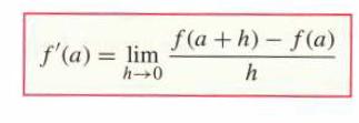
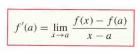
In Exercises 3–8, compute ƒ(a) in two ways, using Eq. (1) and Eq. (2).ƒ(x) = x2 + 9x, a = 0 f'(a) = lim h→0 f(a+h)-f(a) h
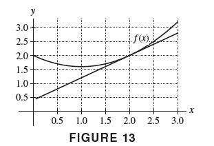
In Exercises 9–12, refer to Figure 13.Estimate ƒ(2 + h) − ƒ(2)/h for h = −0.5. What does this quantity represent? Is it larger or smaller than ƒ'(2)? Explain. 3.0 2.5 2.0 1.5 1.0 0.5 y 0.5 1.0 f(x). 1.5 2.0 2.5 3.0 FIGURE 13 ·x
In Exercises 29–46, use the limit definition to compute ƒ'(a) and find an equation of the tangent line.ƒ(x) = 1/√2x + 1, a = 4
In Exercises 29–46, use the limit definition to compute ƒ'(a) and find an equation of the tangent line.ƒ(t) =√t2 + 1, a = 3
In Exercises 29–46, use the limit definition to compute ƒ'(a) and find an equation of the tangent line.ƒ(x) = x−2, a = −1
In Exercises 29–46, use the limit definition to compute ƒ'(a) and find an equation of the tangent line.ƒ(x) = 1/x2 + 1, a = 0
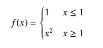
Show that ƒ is not differentiable and x = 1 and has a corner in its graph there. f(x) = (1 (+2 x ≤ 1 x² x ≥ 1
In Exercises 29–46, use the limit definition to compute ƒ'(a) and find an equation of the tangent line.ƒ(t) = t−3, a = 1
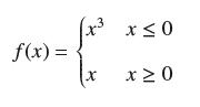
Show that ƒ is not differentiable and x = 0 and has a corner in its graph there. f(x) = x ≤0 x≥0
In Exercises 49–51, sketch a graph of ƒ and identify the points c such that ƒ'(c) does not exist. In which cases is there a corner at c?ƒ(x) = |x + 3|
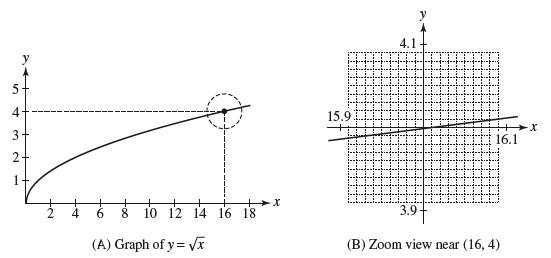
Figure 15(A) shows the graph of ƒ(x) = √x. The close-up in Figure 15(B) shows that the graph is nearly a straight line near x = 16. Estimate the slope of this line and take it as an estimate for ƒ'(16). Then compute ƒ'(16) with the limit definition and compare with your estimate. 5 4 3 N P 10
In Exercises 49–51, sketch a graph of ƒ and identify the points c such that ƒ'(c) does not exist. In which cases is there a corner at c?ƒ(x) = x2/5
In Exercises 49–51, sketch a graph of ƒ and identify the points c such that ƒ'(c) does not exist. In which cases is there a corner at c?ƒ(x) = |x2 − 4|
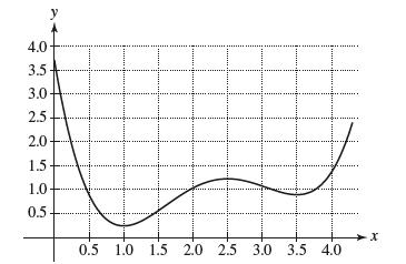
Determine the intervals along the x-axis on which the derivative in Figure 16 is positive. y 4.0 3.5 3.0 2.5 2.0- 1.5 1.0 0.5 0.5 1.0 1.5 2.0 2.5 3.0 3.5 4.0 →Х
Let ƒ(x) = 4/1 + 2x . Plot ƒ over [−2, 2]. Then zoom in near x = 0 until the graph appears straight, and estimate the slope ƒ'(0).
Let ƒ(x) = cot x. Estimate ƒ'(π/2) graphically by zooming in on a plot of ƒ near x = π/2.
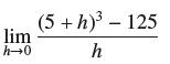
In Exercises 57–62, each limit represents a derivative ƒ'(a). Find ƒ(x) and a. lim h→0 (5 + h)³ - 125 h
Sketch the graph of ƒ(x) = sin x on [0, π] and guess the value of ƒ'(π/2). Then calculate the difference quotient at x = π/2 for two small positive and negative values of h. Are these calculations consistent with your guess?
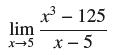
In Exercises 57–62, each limit represents a derivative ƒ'(a). Find ƒ(x) and a. ²³-125 lim x+5 x-5
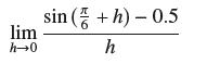
In Exercises 57–62, each limit represents a derivative ƒ'(a). Find ƒ(x) and a. lim h→0 sin (+h)-0.5 h
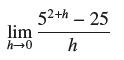
In Exercises 57–62, each limit represents a derivative ƒ'(a). Find ƒ(x) and a. lim h→0 52th - 25 h
In Exercises 57–62, each limit represents a derivative ƒ'(a). Find ƒ(x) and a. lim h→0 5h-1 h
Apply the method of Example 6 to ƒ'(x) = sin x to determine ƒ'(π/4) accurately to four decimal places. EXAMPLE 6 Estimate the derivative of f(x) = sin x at x =.
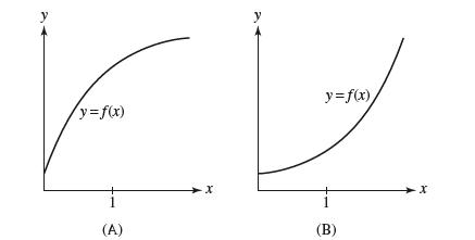
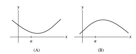
For each graph in Figure 17, determine whether ƒ'(1) is larger or smaller than the slope of the secant line between x = 1 and x = 1 + h for h > 0. Explain. y y= f(x) 1 (A) X y y = f(x), 1 (B) X
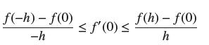
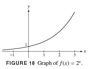
Refer to the graph of ƒ(x) = 2x in Figure 18.(a) Explain graphically why, for h > 0,(b) Use (a) to show that 0.69314 ≤ ƒ'(0) ≤ 0.69315.(c) Similarly, compute ƒ'(x) to four decimal places for x = 1, 2, 3, 4.(d) Now compute the ratios ƒ'(x)/ƒ'(0) for x = 1, 2, 3, 4. Can you guess an
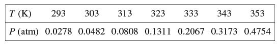
The vapor pressure of water at temperature T (in kelvins) is the atmospheric pressure P at which no net evaporation takes place. Use the following table to estimate the indicated derivatives using the difference quotient approximation.Estimate P'(T) for T = 303, 323, 343. (Include proper units on
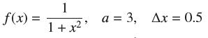
Verify that P = (1, 1/2) lies on the graphs of both ƒ(x) = 1/(1 + x2) and L(x) = 1/2 + m(x − 1) for every slope m. Plot y = ƒ(x) and y = L(x) on the same axes for several values of m until you find a value of m for which y = L(x) appears tangent to the graph of ƒ. What is your estimate for
Plot ƒ(x) = xx and y = 2x + a on the same set of axes for several values of a until the line becomes tangent to the graph. Then estimate the value c such that ƒ'(c) = 2.
Estimate P'(t) for t = 1997, 2001, 2005, 2009. (Include proper units on the derivative.)
Estimate P'(t) for t = 1999, 2003, 2007, 2011. (Include proper units on the derivative.)
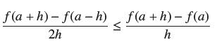
Which of the two functions in Figure 21 satisfies the inequalityfor h > 0? Explain in terms of secant lines. f(a+h)-f(a-h) f(a+h)-f(a) 2h h
(a) Show that the symmetric difference quotient ƒ(a + h) − ƒ(a − h)/2h is the slope of the secant line to the graph of ƒ from x = a − h to x = a + h. (Include an illustration.)(b) Prove that the symmetric difference quotient is the average of the slopes of the secant lines from x to x + h
With P(T) as in Exercises 71 and 72, estimate P(T) for T = 303, 313, 333, 343, now using the SDQ.Data From Exercises 71The vapor pressure of water at temperature T (in kelvins) is the atmospheric pressure P at which no net evaporation takes place. Use the following table to estimate the indicated
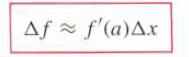
Use Eq. (1) to estimate Δƒ = ƒ(3.02) − ƒ(3).ƒ(x) = x2 Δf ~ f'(α)Δ.χ
Use Eq. (1) to estimate Δƒ = ƒ(3.02) − ƒ(3).ƒ(x) = x4 Δf ~ f'(α)Δ.χ
Use Eq. (1) to estimate Δƒ = ƒ(3.02) − ƒ(3).ƒ(x) = x−1 Δf ~ f'(α)Δ.χ
Use Eq. (1) to estimate Δƒ = ƒ(3.02) − ƒ(3). Δf ~ f'(α)Δ.χ
Use Eq. (1) to estimate Δƒ = ƒ(3.02) − ƒ(3).ƒ(x) = √x + 6 Δf ~ f'(α)Δ.χ
Use Eq. (1) to estimate Δƒ = ƒ(3.02) − ƒ(3).ƒ(x) = tan πx/3 Δf ~ f'(α)Δ.χ
Use Eq. (1) to estimate Δƒ. Use a calculator to compute both the error and the percentage error.ƒ(x) = √1 + x, a = 3, Δx = 0.2 Δf ~ f'(α)Δ.x
The cube root of 64 is 4. How much smaller is the cube root of 63.6? Estimate using the Linear Approximation.
Use Eq. (1) to estimate Δƒ. Use a calculator to compute both the error and the percentage error.ƒ(x) = 2x2 − x, a = 5, Δx = −0.4 Δf ~ f'(α)Δ.x
Use Eq. (1) to estimate Δƒ. Use a calculator to compute both the error and the percentage error. Δf ~ f'(α)Δ.x
Use Eq. (1) to estimate Δƒ. Use a calculator to compute both the error and the percentage error. Δf ~ f'(α)Δ.x
Using Linear Approximation, estimate Δƒ for a change in x from x = a to x = b. Use the estimate to approximate ƒ(b), and find the error using a calculator.ƒ(x) = √x, a = 25, b = 26
Using Linear Approximation, estimate Δƒ for a change in x from x = a to x = b. Use the estimate to approximate ƒ(b), and find the error using a calculator.ƒ(x) = x1/4, a = 16, b = 16.5
Using Linear Approximation, estimate Δƒ for a change in x from x = a to x = b. Use the estimate to approximate ƒ(b), and find the error using a calculator.ƒ(x) = 1/√x , a = 100, b = 101
Using Linear Approximation, estimate Δƒ for a change in x from x = a to x = b. Use the estimate to approximate ƒ(b), and find the error using a calculator.ƒ(x) = 1/√x , a = 100, b = 98
Using Linear Approximation, estimate Δƒ for a change in x from x = a to x = b. Use the estimate to approximate ƒ(b), and find the error using a calculator.ƒ(x) = x1/3, a = 8, b = 9
Using Linear Approximation, estimate Δƒ for a change in x from x = a to x = b. Use the estimate to approximate ƒ(b), and find the error using a calculator.ƒ(x) = x1/3, a = 27, b = 30
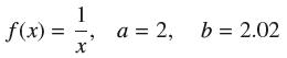
Find the linearization at x = a and then use it to approximate ƒ(b). f(x) = 1 X a = 2, b = 2.02
Find the linearization at x = a and then use it to approximate ƒ(b).ƒ(x) = x4, a = 1, b = 0.96
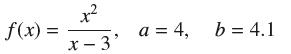
Find the linearization at x = a and then use it to approximate ƒ(b). f(x) = x² x-3' a = 4, b = 4.1
Find the linearization at x = a and then use it to approximate ƒ(b).ƒ(x) = sin2 x, a = π/4, b = 1.1π/4
Find the linearization at x = a and then use it to approximate ƒ(b).ƒ(x) = (1 + x)−1/2, a = 0, b = 0.08
Find the linearization at x = a and then use it to approximate ƒ(b).ƒ(x) = (1 + x)−1/2, a = 3, b = 2.88
Find the linearization at x = a and then use it to approximate ƒ(b).ƒ(x) = e√x, a = 1, b = 0.85
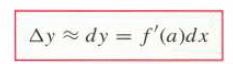
Estimate Δy using differentials [Eq. (3)].y = cos x, a = π/6, dx = 0.014 Ay dy = f'(a)dx ~
Find the linearization at x = a and then use it to approximate ƒ(b).ƒ(x) = ex ln x, a = 1, b = 1.02
Estimate Δy using differentials [Eq. (3)].y = tan2 x, a = π/4, dx = −0.02 Ay dy= f'(a)dx ~
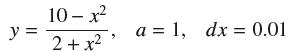
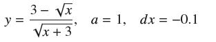
Estimate Δy using differentials [Eq. (3)]. Ay dy= f'(a)dx ~
Estimate Δy using differentials [Eq. (3)]. Ay dy= f'(a)dx ~
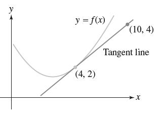
Estimate ƒ(4.03) for ƒ(x) as in Figure 9. y = f(x) (4,2) (10,4) Tangent line -X
At a certain moment, an object in linear motion has velocity 100 m/s. Estimate the distance traveled over the next quarter-second, and explain how this is an application of the Linear Approximation.
Estimate sin 61° − sin 60° using the Linear Approximation. Hint: Express Δθ in radians.
Box office revenue at a multiplex cinema in Paris is R(p) = 3600p − 10p3 euros per showing when the ticket price is p euros. Calculate R(p) for p = 9 and use the Linear Approximation to estimate ΔR if p is raised or lowered by 0.5 euro.
The stopping distance for an automobile is F(s) = 1.1s + 0.054s2 ft, where s is the speed in mph. Use the Linear Approximation to estimate the change in stopping distance per additional mph when s = 35 and when s = 55.
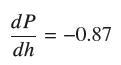
The atmospheric pressure P at altitude h = 20 km is P = 5.5 kilopascals. Estimate P at altitude h = 20.5 km assuming that dP dh = -0.87
At a certain moment, the temperature in a snake cage satisfies dT/dt = 0.008°C/s. Estimate the rise in temperature over the next 10 s.
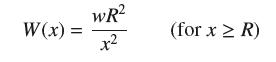
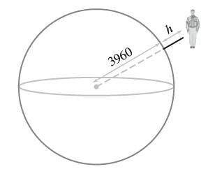
Newton’s Law of Gravitation shows that if a person weighs w pounds on the surface of the earth, then his or her weight at distance x from the center of the earth iswhere R = 3960 miles is the radius of the earth (Figure 10).(a) Show that the weight lost at altitude h miles above the earth’s
The resistance R of a copper wire at temperature T = 20°C is R = 15 Ω. Estimate the resistance at T = 22°C, assuming that dR/dTΙT=20 = 0.06 Ω/°C.
Using Exercise 41(a), estimate the altitude at which a 130-lb pilot would weigh 129.5 lb.Data From Exercise 41 (a)(a) Show that the weight lost at altitude h miles above the earth’s surface is approximately ΔW ≈ −(0.0005w)h. Use the Linear Approximation with dx = h.
A stone tossed vertically into the air with initial velocity v cm/s reaches a maximum height of h = v2/1960 cm.(a) Estimate Δh if v = 700 cm/s and Δv = 1 cm/s.(b) Estimate Δh if v = 1000 cm/s and Δv = 1 cm/s.(c) In general, does a 1-cm/s increase in v lead to a greater change in h at low or
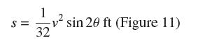
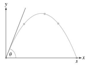
Use the following fact derived from Newton’s Laws: An object released at an angle θ with initial velocity v ft/s travels a horizontal distanceA player located 18.1 ft from the basket launches a successful jump shot from a height of 10 ft (level with the rim of the basket), at an angle θ = 34°
The side s of a square carpet is measured at 6 m. Estimate the maximum error in the area A of the carpet if s is accurate to within 2 cm.
In the notation of Exercise 49, assume that a measurement yields V = 4. Estimate the maximum allowable error in V if P must have an error of less than 0.2 atm.Data From Exercise 49The volume (in liters) and pressure P (in atmospheres) of a certain gas satisfy PV = 24. A measurement yields V = 4
The dosage D of diphenhydramine for a dog of body mass w kg is D = 4.7w2/3 mg. Estimate the maximum allowable error in w for a cocker spaniel of mass w = 10 kg if the percentage error in D must be less than 3%.
A golfer hits a golf ball at an angle of θ = 23° with initial velocity v = 120 ft/s.(a) Estimate Δs if the ball is hit at the same velocity but the angle is increased by 3°.(b) Estimate Δs if the ball is hit at the same angle but the velocity is increased by 3 ft/s.
Approximate f (2) if the linearization of f (x) at a = 2 is L(x) = 2x + 4?
Compute the linearization of ƒ(x) = 3x − 4 at a = 0 and a = 2. Prove more generally that a linear function coincides with its linearization at x = a for all a.
Estimate √16.2 using the linearization L(x) of ƒ(x) = √x at a = 16. Plot f and L on the same set of axes and determine whether the estimate is too large or too small.
Estimate 1/√15 using a suitable linearization of ƒ(x) = 1/√x. Plot f and L on the same set of axes and determine whether the estimate is too large or too small. Use a calculator to compute the percentage error.
Approximate using linearization and use a calculator to compute the percentage error.1/√17
Approximate using linearization and use a calculator to compute the percentage error.1/101
Approximate using linearization and use a calculator to compute the percentage error.1/(10.03)2
Approximate using linearization and use a calculator to compute the percentage error.(17)1/4
Approximate using linearization and use a calculator to compute the percentage error.(64.1)1/3
Approximate using linearization and use a calculator to compute the percentage error.(1.2)5/3
Approximate using linearization and use a calculator to compute the percentage error.tan(0.04)
Approximate using linearization and use a calculator to compute the percentage error.cos (3.1/4)
Approximate using linearization and use a calculator to compute the percentage error.(3.1)/2/sin(3.1/2)
Compute the linearization L(x) of ƒ(x) = x2 − x3/2 at a = 4. Then plot ƒ − L and find an interval I around a = 4 such that |ƒ(x) − L(x)| ≤ 0.1 for x ∈ I.
Show that the Linear Approximation to ƒ(x) = √x at x = 9 yields the estimate √9 + h − 3 ≈ 1/6 h. Set K = 0.01 and show that |ƒ"(x)| ≤ K for x ≥ 9. Then verify numerically that the error E satisfies Eq. (5) for h = 10−n, for 1 ≤ n ≤ 4. ΕΣ-Κ (Δ.)2 E <
The Linear Approximation to ƒ(x) = tan x at x = π/4 yields the estimate tan π/4 + h − 1 ≈ 2h. Set K = 6.2 and show, using a plot, that |ƒ"(x)| ≤ K for x ∈ [π/4, π/4 + 0.1]. Then verify numerically that the error E satisfies Eq. (5) for h = 10−n, for 1 ≤ n ≤ 4. 1 ΕΣ-Κ
Apply the method of Exercise 69 to P = (0.5, 1) on y5 + y − 2x = 1 to estimate the y-coordinate of the point on the curve where x = 0.55.
Apply the method of Exercise 69 to P = (−1, 2) on y4 + 7xy = 2 to estimate the solution of y4 − 7.7y = 2 near y = 2.
Show that for any real number k, (1 + Δx)k ≈ 1 + kΔx for small Δx. Estimate (1.02)0.7 and (1.02)−0.3.
Let Δƒ= ƒ(1 + h) − ƒ(1), where ƒ(x) = x−1. Show directly that E = |Δƒ − ƒ'(1)h| is equal to h2/(1 + h). Then prove that E ≤ 2h2 if −1/2 ≤ h ≤ 1/2. In this case, 1/2 ≤ 1 + h ≤ 3/2.
In Exercises 9–12, refer to Figure 13.Estimate ƒ(1) andƒ'(2). 3.0 2.5 2.0 1.5 1.0 0.5 y 0.5 1.0 f(x). 1.5 2.0 2.5 3.0 FIGURE 13 ·x

Showing 6800 - 6900 of 8339

First
62
63
64
65
66
67
68
69
70
71
72
73
74
75
76
Last

Step by Step Answers

Services

Sitemap
Fun
Definitions
Become Tutor
Used Textbooks
Study Help Categories
Recent Questions
Expert Questions
Campus Wear
Sell Your Books

Company Info

Security
Copyrights
Privacy Policy
Terms & Conditions
SolutionInn Fee
Scholarship
Online Quiz
Give Feedback, Get Rewards

Get In Touch

About Us
Contact Us
Career
Jobs
FAQ
Student Discount
Campus Ambassador

Secure Payment

Download Our App

© 2026 SolutionInn. All Rights Reserved