New Semester
Started
Get
50% OFF
Study Help!
--h --m --s
Claim Now
Question Answers
Textbooks
Find textbooks, questions and answers
Oops, something went wrong!
Change your search query and then try again
S
Books
FREE
Study Help
Expert Questions
Accounting
General Management
Mathematics
Finance
Organizational Behaviour
Law
Physics
Operating System
Management Leadership
Sociology
Programming
Marketing
Database
Computer Network
Economics
Textbooks Solutions
Accounting
Managerial Accounting
Management Leadership
Cost Accounting
Statistics
Business Law
Corporate Finance
Finance
Economics
Auditing
Tutors
Online Tutors
Find a Tutor
Hire a Tutor
Become a Tutor
AI Tutor
AI Study Planner
NEW
Sell Books
Search
Search
Sign In
Register
study help
business
introduction to probability statistics
Introduction To Probability And Statistics 3rd Edition William Mendenhall - Solutions
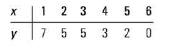
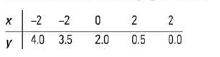
12.56 Reverse the slope of the line in Exercise 12.55 by reordering the y observations, as follows:Repeat the steps of Exercise 12.55. Notice the change in the sign of r and the relationship between the values of r of Exercise 12.55 and this exercise. y 1 2 3 3 4 5 6 0 2 3 5 5 7
12.55 You are given these data:a. Plot the six points on graph paper.b. Calculate the sample coefficient of correlation and interpret.c. By what percentage was the sum of squares of deviations reduced by using the least-squares pre- dictor = a + bx rather than as a predictor of y? x y 1 2 3 4 5 6 7
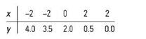
12.54 You are given these data:a. Plot the data points. Based on your graph, what will be the sign of the sample correlation coefficient?b. Calculate r and r and interpret their values. x -2 -1 0 1 2 y 2 2 3 4 4
12.53 What value does r assume if all the data points fall on the same straight line in these cases?a. The line has positive slope.b. The line has negative slope.
12.52 Describe the significance of the algebraic sign and the magnitude of r.
12.51 How does the coefficient of correlation measure the strength of the linear relationship between two variables y and x?
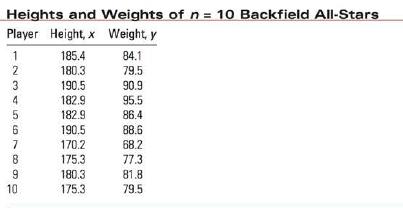
Refer to the height and weight data in Example 12.7. The correlation of height and weight was calculated to be r = 0.8261. Is this correlation significantly different from 0?
The heights and weights of n = 10 offensive backfield football players are randomly selected from a county's football all-stars. Calculate the correlation coefficient for the heights (in centimetres) and weights (in kilograms) given in Table 12.4. Heights and Weights of n = 10 Backfield All-Stars
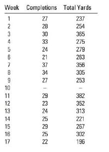
12.50 Drew Brees, continued Refer to Exercise 12.49.a. Estimate the average number of passing yards for games in which Brees throws 20 completed passes using a 95% confidence interval.b. Predict the actual number of passing yards for games in which Brees throws 20 completed passes using a 95%
12.49 Drew Brees The number of passes completed and the total number of passing yards for Drew Brees, quarterback for the New Orleans Saints, were recorded for the 16 regular games in the 2010 football season. 10 He had no games in week 10 and no data was reported.a. What is the least-squares line
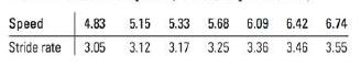
12.48 Stride Rate, continued Refer to Exercise 12.47.a. Estimate the average stride rate if the speed is 5.8 metres per second using a 95% confidence interval.b. Predict the actual number of the stride rate if the speed is 5.8 metres per second using a 95% prediction interval.c. Would it be
12.47 Stride Rate One measure of form for a runner is stride rate, defined as the number of steps per second. A runner is considered to be efficient if the stride rate is close to optimum. The stride rate is related to speed; the greater the speed, the greater the stride rate. In a study of some
12.46 Strawberries III The following data (Exercises 12.18 and 12.28) were obtained in an experiment relating the dependent variable, y (texture of strawberries), with x (coded storage temperature).a. Estimate the expected strawberry texture for a coded storage temperature of x = -1. Use a 99%
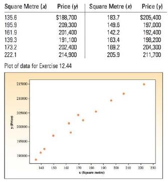
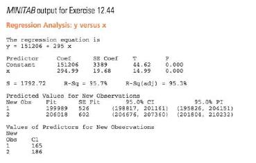
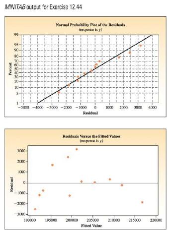
12.45 Housing Prices II Refer to Exercise 12.44 and data set EX1244.a. Estimate the average increase in the price for an increase of 1 m for houses sold in the city. Use a 99% confidence interval. Interpret your estimate.b. A real estate salesperson needs to estimate the average sales price of
12.44 Housing Prices If you try to rent an apartment or buy a house, you find that real estate representatives establish apartment rents and house prices on the basis of square footage of heated floor space. The data in the table give the square footages and sales prices of n = 12 houses randomly
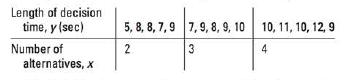
12.43 What to Buy? A marketing research experiment was conducted to study the relationship between the length of time necessary for a buyer to reach a decision and the number of alternative package designs of a product presented. Brand names were eliminated from the packages to reduce the effects
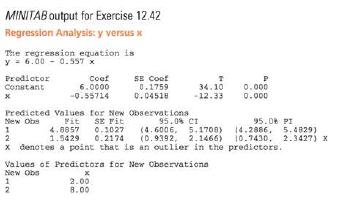
12.42 Refer to Exercise 12.7. Portions of the MINITAB printout are shown here.a. Find a 95% confidence interval for the average value of y when x = 2.b. Find a 95% prediction interval for some value of y to be observed in the future when x = 2.c. The last line in the third section of the printout
12.41 Refer to Exercise 12.6.a. Estimate the average value of y when x = 1, using a 90% confidence interval.b. Find a 90% prediction interval for some value of y to be observed in the future when x = 1.
Prior to fitting a line to the calculus grade-achievement score data, you may have thought that a score of 0 on the achievement test would predict a grade of 0 on the cal- culus test. This implies that we should fit a model with a equal to 0. Do the data support the hypothesis of a 0 intercept?
A student took the achievement test and scored 50 but has not yet taken the calculus test. Using the information in Example 12.1, predict the calculus grade for this student with a 95% prediction interval.
Use the information in Example 12.1 to estimate the average calculus grade for students whose achievement score is 50, with a 95% confidence interval.
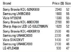
12.40 LCD TVs As technology improves, the choice of televisions becomes more compli- cated. Should you choose an LCD TV, an LED TV, or a plasma TV? Does the price of an LCD TV depend on the size of the screen? In the table below, Consumer Reports gives the prices and screen sizes for the top 10 LCD
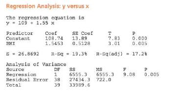
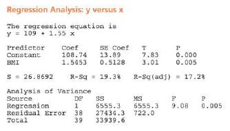
12.39 Systolic Blood Pressure (SBP) and Body Mass Index (BMI), again Refer to Exercise 12.29. The MINITAB printout is reproduced here.a. What assumptions must be made about the distribution of the random error, e?b. What is the best estimate of o, the variance of the random error, e?c. Use the
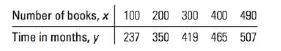
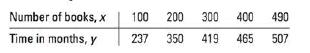
12.38 Professor Asimov, again Refer to Exercise 12.9, in which the number of books x written by Isaac Asimov are related to the number of months y he took to write them. A plot of the data is shown.a. Can you see any pattern other than a linear relationship in the original plot?b. The value of r
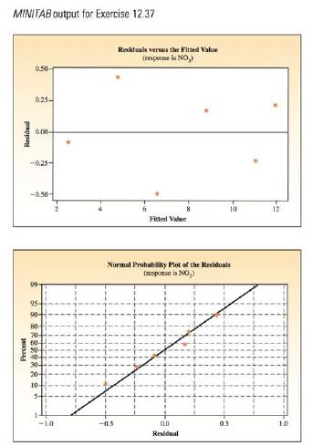
12.37 Air Pollution Refer to Exercise 12.23, in which an air pollution monitor's response to ozone was recorded for several different concentrations of ozone. Use the MINITAB residual plots to comment on the validity of the regression assumptions. Percent 99 MINITAB output for Exercise 12.37
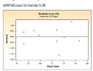
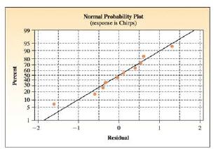
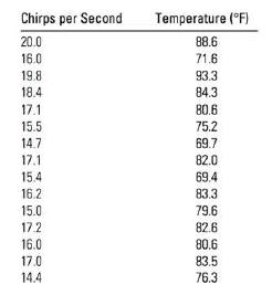
12.36 Chirping Crickets Refer to Exercise 12.24, in which the number of chirps per second for a cricket was recorded at 10 different temperatures. Use the MINITAB diagnostic plots to comment on the validity of the regression assumptions. Residual MINITAB output for Exercise 12.36 Residuals versus
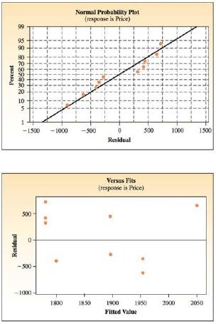
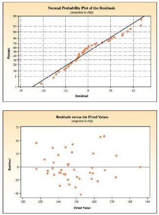
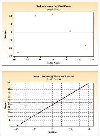
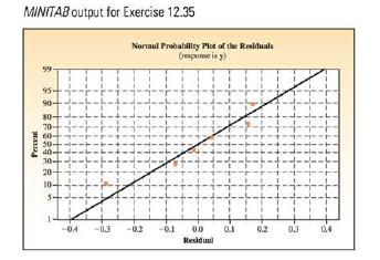
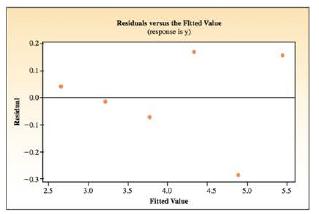
12.35 Refer to the data in Exercise 12.7. The normal probability plot and the residuals versus fitted values plots generated by MINITAB are shown here. Does it appear that any regression assumptions have been violated? Explain. Per MINITAB output for Exercise 12.35 Normal Probability Plot of the
12.34 What diagnostic plot can you use to determine whether the assumption of equal variance has been violated? What should the plot look like when the variances are equal for all values of x?
12.33 What diagnostic plot can you use to determine whether the incorrect model has been used? What should the plot look like if the correct model has been used?
12.32 What diagnostic plot can you use to determine whether the data satisfy the normality assumption? What should the plot look like for normal residuals?
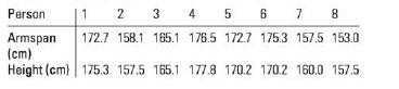
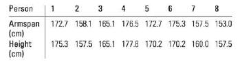
12.31 Armspan and Height II In Exercise 12.17 (data set EX1217), we measured the armspan and height of eight people with the following results:a. Does the data provide sufficient evidence to indicate that there is a linear relationship between armspan and height? Test at the 5% level of
12.30 Systolic Blood Pressure (SBP) and Body Mass Index (BMI), continued Refer to Exercise 12.29.a. Use the MINITAB printout to find the value of the coefficient of determination, 2. Show that P = SSR/Total SS.b. What percentage reduction in the total variation is achieved by the linear regression
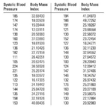
12.29 Systolic Blood Pressure (SBP) and Body Mass Index (BMI) In the case study of Chapter 1 we provided the blood pressure data on 500 persons (both male and females). Here we take a random sample of 40 persons. In the first column the blood pressure (y) and in the second column body mass index
12.28 Strawberries II The following data (Exercise 12.18 and data set EX1218) were obtained in an experiment relating the dependent variable, y (texture of strawberries), with x (coded storage temperature). Use the information from Exercise 12.18 to answer the following questions:a. What is the
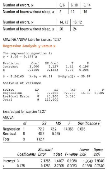
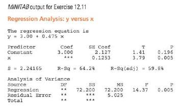
12.27 Sleep Deprivation III Refer to the sleep deprivation experiment described in Exercise 12.11 and data set EX1211. The data and the MINITAB and Excel printouts are reproduced here.a. Do the data present sufficient evidence to indicate that the number of errors is linearly related to the number
12.26 Professor Asimov, continued Refer to the data in Exercise 12.9, relating x, the number of books written by Professor Isaac Asimov, to y, the number of months he took to write his books (in increments of 100). The data are reproduced here.a. Do the data support the hypothesis that = 0? Use the
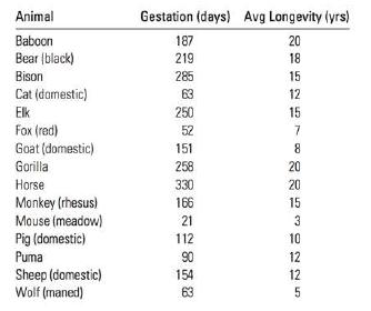
12.25 Gestation Times and Longevity The table below shows the gestation time in days and the average longevity in years for a variety of mammals in captivity.a. If you want to estimate the average longevity of an animal based on its gestation time, which variable is the response variable and which
12.24 Cricket (the insect, not the game) Crickets make their chirping sounds by rapidly sliding one wing over the other. The faster they move their wings, the higher the chirping sound that is produced. Scientists have noticed that crickets move their wings faster in warm temperatures than in cold
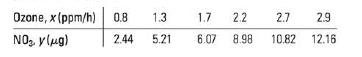
12.23 Air Pollution An experiment was designed to compare several different types of air pollution monitors.4 The monitor was set up, and then exposed to different concentrations of ozone, ranging between 15 and 230 parts per million (ppm) for periods of 8-72 hours. Filters on the monitor were then
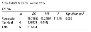
12.22 Refer to Exercise 12.8. The data, along with the Excel analysis of variance table, are reproduced below:a. Do the data provide sufficient evidence to indicate that y and x are linearly related? Use the information in the printout to answer this question at the 5% level of significance.b.
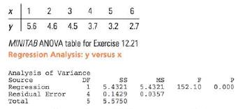
12.21 Refer to Exercise 12.7. The data, along with the MINITAB analysis of variance table, are reproduced below.a. Do the data provide sufficient evidence to indicate that y and x are linearly related? Use the information in the MINITAB printout to answer this question at the 1% level of
12.20 Refer to Exercise 12.19. Find a 95% confi- dence interval for the slope of the line. What does the phrase "95% confident" mean?
12.19 Refer to Exercise 12.6. The data are reproduced below.a. Do the data present sufficient evidence to indicate that y and x are linearly related? Test the hypothesis that =0 at the 5% level of significance.b. Use the ANOVA table to calculate F = MSR/MSE. Verify that the square of the r
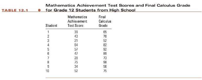
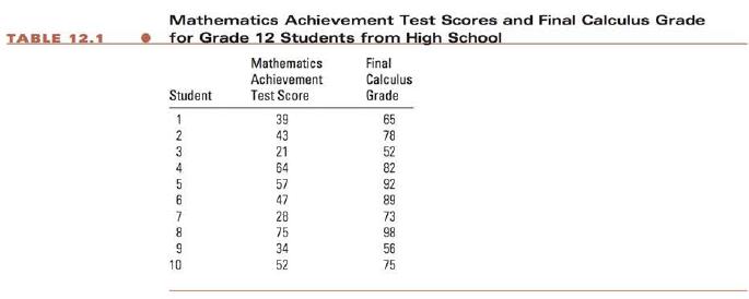
Find a 95% confidence interval estimate of the slope for the calculus grade data in Table 12.1. TABLE 12.1 Mathematics Achievement Test Scores and Final Calculus Grade for Grade 12 Students from High School Mathematics Achievement Final Calculus Student 1 Test Score Grade 39 65 10 23456789O 43 78
Determine whether there is a significant linear relationship between the calculus grades and test scores listed in Table 12.1. Test at the 5% level of significance. TABLE 12.1 Mathematics Achievement Test Scores and Final Calculus Grade for Grade 12 Students from High School Mathematics
12.18 Strawberries The following data were obtained in an experiment relating the dependent variable, y (texture of strawberries), with x (coded storage temperature).a. Find the least-squares line for the data.b. Plot the data points and graph the least-squares line as a check on your
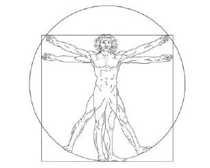
12.17 Armspan and Height Leonardo daVinci (1452-1519) drew a sketch of a man, indicating that a person's armspan (measuring across the back with your arms outstretched to make a "t") is roughly equal to the person's height. To test this claim, we measured eight people with the following results:a.
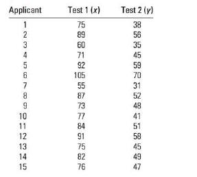
12.16 Test Interviews, continued Refer to Exercise 12.15. Construct the ANOVA table for the linear regression relating y, the score on Test 2, to x, the score on Test 1.
12.15 Test Interviews Of two personnel evaluation techniques available, the first requires a two-hour test interview, while the second can be completed in less than an hour. The scores for each of the 15 individuals who took both tests are given in the next table.a. Construct a scatterplot for the
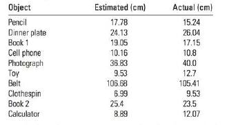
12.14 How Long Is It? How good are you at estimating? To test a subject's ability to estimate sizes, he was shown 10 different objects and asked to estimate their length or diameter. The object was then measured, and the results were recorded in the table below.a. Find the least-squares regression
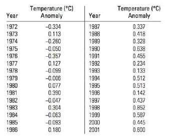
12.13 Global Warming? The following table shows annual mean global surface temperature anomaly for the period 1972 to 2001 provided by the Global Historical Climate Network (GHCN).a. Which of the two variables is the independent variable and which is the dependent variable? Explain your choice.b.
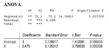
12.12 Sleep Deprivation II Refer to the data given in the sleep deprivation experiment in Exercise 12.11. Answer the questions posed in partsa, b,d, and e of that exercise by completing the following Excel printout: ANOVA F Significance F df S8 MS Regression 72.2 72.2 14.36816 Residual Total 5.025
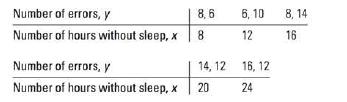
12.11 Sleep Deprivation A study was conducted to determine the effects of sleep deprivation on people's ability to solve problems without sleep. A total of 10 subjects participated in the study, two at each of five sleep deprivation levels 8, 12, 16, 20, and 24 hours. After his or her specified
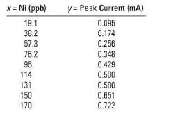
12.10 A Chemical Experiment Using a chemical procedure called differential pulse polarography, a chemist measured the peak current generated (in microamperes) when a solution containing a given amount of nickel (in parts per billion) is added to a buffer:a. Use the data entry method for your
12.9 Professor Asimov Professor Isaac Asimov was one of the most prolific writers of all time. Prior to his death, he wrote nearly 500 books during a 40-year career. In fact, as his career progressed, he became even more productive in terms of the number of books written within a given period of
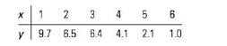
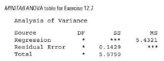
12.7 Six points have these coordinates:a. Find the least-squares line for the data.b. Plot the six points and graph the line. Does the line appear to provide a good fit to the data points?c. Use the least-squares line to predict the value of y when x = 3.5.d. Fill in the missing entries in the
12.5 What is the difference between deterministic and probabilistic mathematical models?
12.4 Give the equation and graph for a line with y-intercept equal to -3 and slope equal to 1.
12.3 Give the equation and graph for a line with y-intercept equal to 3 and slope equal to -1.
12.1 Graph the line corresponding to the equation y=2x+1 by graphing the points corresponding to x = 0, 1, and 2. Give the y-intercept and slope for the line.
Find the least-squares prediction line for the calculus grade data in Table 12.1. TABLE 12.1 Mathematics Achievement Test Scores and Final Calculus Grade for Grade 12 Students from High School Mathematics Achievement Final Calculus Student Test Score Grade 1 39 65 10 23456789O 43 78 21 52 64 82 57
13.27 Advertising and Sales, continued Refer to Exercise 13.26. Use a computer software package to perform the multiple regression analysis and obtain diagnostic plots if possible.a. Comment on the fit of the model, using the analysis of variance F test, R2, and the diagnostic plots to check the
Suppose that a response variable Y is related to four predictor variables, X1, X2, X3, and x4, so that k = 4. 1. Enter the observed values of y and each of the k = 4 predictor variables into the first (k + 1) columns of a MINITAB worksheet. Once this is done, the main inferential tools for multiple
Suppose that a response variable Y is related to four predictor variables, x1, x2, x3, and x4, so that k = 4. 1. Enter the observed values of y and each of the k = 4 predictor variables into the first (k + 1) columns of an Excel spreadsheet. (NOTE: In order for the mul- tiple regression analysis to
Refer to the real estate data of Example 13.2 that relate the listed selling price y to the square metres of living area x, the number of floors x2, the number of bedrooms X3, and the number of bathrooms, x4. The realtor suspects that square metres of liv- ing area is the most important predictor
13.19 A multiple linear regression model involv- ing one qualitative and one quantitative independent variable produced this prediction equation: y= 12.6+0.54x1-1.2x1x2 + 3.9xa. Which of the two variables is the quantitative variable? Explain.b. If x, can take only the values 0 or 1, find the two
13.18 Suppose E(Y) is related to two predictor variables x and x2 by the equation E(Y) 3+x 2x2 + x1x2a. Graph the relationship between E(Y) and x, when x20. Repeat for x2 = 2 and for x2 = -2.b. Repeat the instructions of part a for the model E(Y)=3+x-2x2c. Note that the equation for part a is
13.17 Production Yield Suppose you wish to predict production yield y as a function of several independent predictor variables. Indicate whether each of the following independent variables is qualitative or quantitative. If qualitative, define the appropriate dummy variable(s).a. The prevailing
Refer to Example 13.6. Do the data provide sufficient evidence to indicate that the annual rate of increase in male junior faculty salaries exceeds the annual rate of in- crease in female junior faculty salaries? That is, do the data provide sufficient evidence to indicate that the slope of the
A study was conducted to examine the relationship between university salary Y, the number of years of experience of the faculty member, and the gender of the faculty member. If you expect a straight-line relationship between mean salary and years of experience for both men and women, write the
13.11 University Textbooks II Refer to Exercise 13.10.a. Use the values of SSR and Total SS to calculate R. Compare this value with the value given in the printout.b. Calculate R(adj). When would it be appropriate to use this value rather than R to assess the fit of the model?c. The value of R(adj)
13.8 Refer to Exercise 13.5.a. Suppose that the relationship between E(Y) and x is a straight line. What would you know about the value of B?b. Do the data provide sufficient evidence to indicate curvature in the relationship between y and x?
13.7 Refer to Exercise 13.5.a. What is your estimate of the average value of y when x = 0?b. Do the data provide sufficient evidence to indicate that the average value of y differs from 0 when x = 0?
13.6 Refer to Exercise 13.5.a. What is the prediction equation?b. Graph the prediction equation over the interval 0 x 6.
13.3 Suppose that you fit the model E(Y) Bo+Bx + B2x2 + B3x3 to 15 data points and found F equal to 57.44.a. Do the data provide sufficient evidence to indicate that the model contributes information for the pre- diction of y? Test using a 5% level of significance.b. Use the value of F to calculate
13.2 Refer to Exercise 13.1.a. Graph the relationship between E(Y) and x2 when x=0. Repeat for x = 1 and for x = 2.b. What relationship do the lines in part a have to one another?c. Suppose, in a practical situation, you want to model the relationship between E(Y) and two predictor variables x and
13.1 Suppose that E(Y) is related to two predictor variables, X, and X2, by the equation E(Y)=3+x1-2x2a. Graph the relationship between E(Y) and x, when x2 = 2. Repeat for x2 = 1 and for x2 = 0.b. What relationship do the lines in part a have to one another?
Refer to the data on grocery retail outlet productivity and outlet size in Example 13.3. MINITAB was used to fit a quadratic model to the data and to graph the quadratic predic- tion curve, along with the plotted data points. Discuss the adequacy of the fitted model.
Suppose you want to relate a random variable Y to two independent variables x and x2. The multiple regression model is Y=Bo+B1x+B2x2 + with the mean value of y given as E(Y) Bo+B+ Bx2
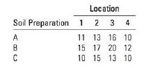
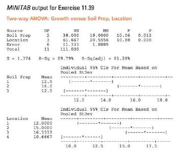
11.39 Slash Pine Seedings An experiment was conducted to determine the effects of three methods of soil preparation on the first-year growth of slash pine seedlings. Four locations (provincial forest lands) were selected, and each location was divided into three plots. Since it was felt that soil
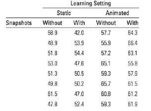
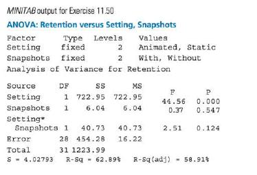
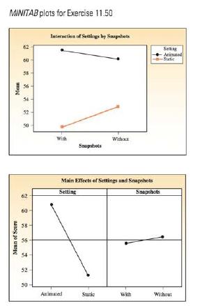
11.50 Animation Helps? To explore ways to increase the educational experience using animation versus static images in a learning environment, Cyril Rebetez and colleagues ran a factorial experiment that measured the retention of information under four factorial conditions: with animation or without
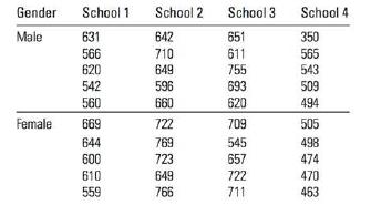
11.51 Standardized Test Scores A local school board was interested in comparing test scores on a standarized reading test for Grade 3 students in its district. It selected a random sample of five male and five female Grade 3 students at each of four different elementary schools in the district and
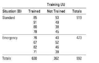
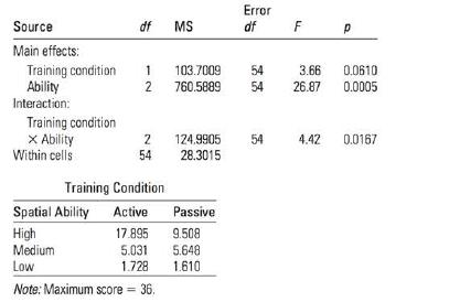
11.52 Management Training An experiment was conducted to investigate the effect of manage- ment training on the decision-making abilities of supervisors in a large corporation. Sixteen supervi- sors were selected, and eight were randomly chosen to receive managerial training. Four trained and four
11.53 Management Training, continued Refer to Exercise 11.52. The data for this experiment are shown in the table.a. Construct the ANOVA table for this experiment.b. Is there a significant interaction between the presence or absence of training and the type of decision-making situation? Test at the
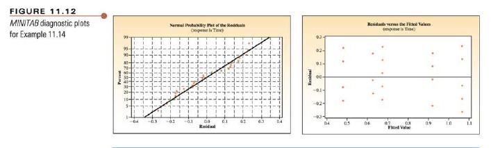
The data from Example 11.4 involving breakfast and the attention spans of three groups of elementary students were analyzed using MINITAB. The graphs in Figure 11.12, gen- erated by MINITAB, are the normal probability plot and the residuals versus fit plot for this experiment. Look at the
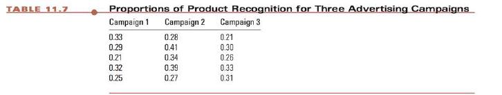
A company plans to promote a new product by using one of three advertising cam- paigns. To investigate the extent of product recognition from these three campaigns, 15 market areas were selected and 5 were randomly assigned to each advertising plan. At the end of the ad campaigns, random samples of
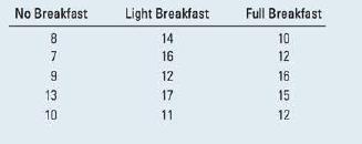
Completely Randomized Design Refer to the breakfast study in Example 11.4, in which the effect of nutrition on attention span (in minutes) was studied.1. Enter the data into columns A, B, and C of an Excel spreadsheet with one sample per column. 2. Use Data Data Analysis Anova: Single Factor to
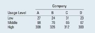
Randomized Block Design Refer to the cell phone study in Example 11.9, in which the effect of usage level on cost (in dollars) was studied for four different companies. 1. Enter the data into columns A-E of an Excel spreadsheet, using column A for usage labels and row 1 for company labels, just as
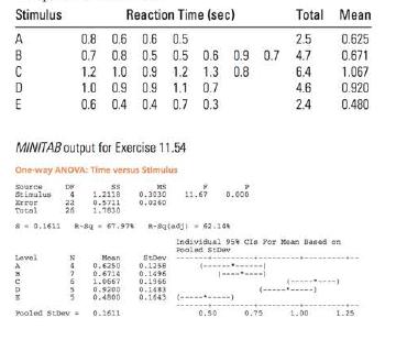
11.54 Reaction Times vs. Stimuli Twenty-seven people participated in an experi- ment to compare the effects of five different stimuli on reaction time. The experiment was run using a com- pletely randomized design, and, regardless of the results of the analysis of variance, the experimenters wanted
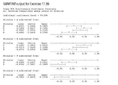
11.55 Refer to Exercise 11.54. Use this MINITAB output to identify the differences in the treatment means. MINITAB output for Exercise 11.55 Tukey 95 Simultaneous Confidence Intervals All Pairwise Comparisons among Levels of stimulus Individual confidence level = 99.296 Stimulus = Stimulus
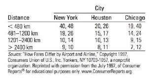
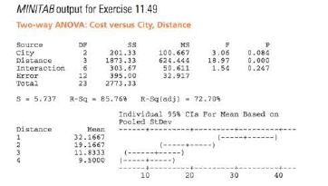
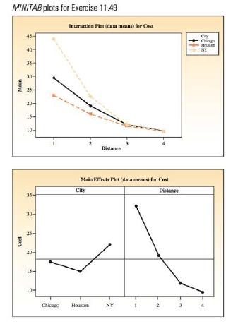
11.49 The Cost of Flying In an attempt to determine what factors affect airfares, a researcher recorded a weighted average of the costs per kilometre for two airports in each of three major U.S. cities for each of four different travel distances. The results are shown in the table.Use the MINITAB
11.48 Terrain Visualization A study was con- ducted to determine the effect of two factors on terrain visualization training for soldiers. During the training programs, participants viewed contour maps of various terrains and then were permitted to view a computer reconstruction of the terrain as
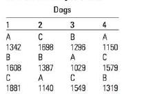
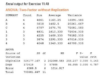
11.40 Digitalis and Calcium Uptake A study was conducted to compare the effects of three levels of digitalis on the levels of calcium in the heart muscles of dogs. Because general level of calcium uptake varies from one animal to another, the tissue for a heart muscle was regarded as a block, and
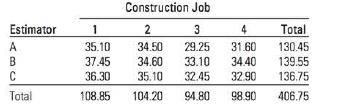
11.41 Bidding on Construction Jobs A building contractor employs three construction engineers, A, B, and C, to estimate and bid on jobs. To determine whether one tends to be a more conservative (or liberal) estimator than the others, the contractor selects four projected construction jobs and has
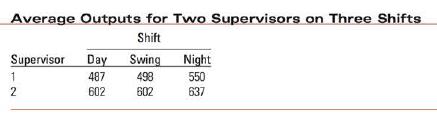
Suppose that the two supervisors are each observed on three randomly selected days for each of the three different shifts. The average outputs for the three shifts are shown in Table 11.4 for each of the supervisors. Look at the relationship between the two factors in the line chart for these
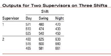
Table 11.6 shows the original data used to generate Table 11.5 in Example 11.12. That is, the two supervisors were each observed on three randomly selected days for each of the three different shifts, and the production outputs were recorded. Analyze these data using the appropriate analysis of
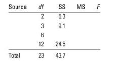
11.43 The analysis of variance table for a 34 factorial experiment, with factor A at three levels and factor B at four levels, and with two observations per treatment, is shown here:a. Fill in the missing items in the table.b. Do the data provide sufficient evidence to indicate that factors A and B
11.44 Refer to Exercise 11.43. The means of two of the factor-level combinations-say, AB and A2B are =8.3 and x2 = 6.3, respectively. Find a 95% confidence interval for the difference between the two corresponding population means.
11.45 The table gives data for a 3 x 3 factorial experiment, with two replications per treatment:a. Perform an analysis of variance for the data, and present the results in an analysis of variance table.b. What do we mean when we say that factors A and B interact?c. Do the data provide sufficient
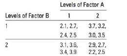
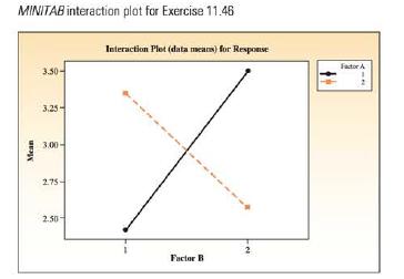
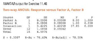
11.46 2 x 2 Factorial The table gives data for a 2 X 2 factorial experiment, with four replications per treatment:a. The accompanying graph was generated by MINITAB. Verify that the four points that connect the two lines are the means of the four observations within each factor-level combination.
Showing 3700 - 3800
of 7136
First
31
32
33
34
35
36
37
38
39
40
41
42
43
44
45
Last
Step by Step Answers