New Semester Started Get 50% OFF Study Help! --h --m --s Claim Now

Question Answers

Textbooks

Find textbooks, questions and answers

Oops, something went wrong!

Change your search query and then try again

Result Not Found

Books FREE
Study Help
Tutors
AI Study Planner NEW
Sell Books

Search
Sign In
Register

study help
engineering
mechanical vibration analysis

Mechanical Vibration Analysis, Uncertainties, And Control 4th Edition Haym Benaroya, Mark L Nagurka, Seon Mi Han - Solutions

Identify the poles and zeros for the following secondorder systems, and discuss system stability:(a) \(\ddot{y}+2 \dot{y}+y=A \cos 3 t\)(b) \(\ddot{y}+\dot{y}+0.1 y=A \cos 3 t\)(c) \(\ddot{y}+300 \dot{y}+10 y=A \cos 3 t\)(d) \(\ddot{y}+2 \dot{y}+y=A_{1} x+A_{2} \dot{x}\)(e) \(\ddot{y}+y=A \cos
For the given transfer functions, determine the governing differential equation of motion:(a) \(T(s)=(2 s+2) /\left(s^{2}+2 s+5\right)\)(b) \(T(s)=(s-1) /\left(3 s^{2}+4\right)\)(c) \(T(s)=(s+1) /\left(s^{2}+s+1\right)\).
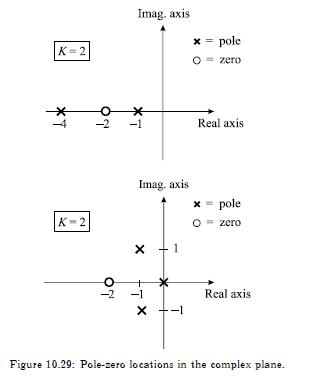
For a gain factor \(K=2\), use the pole-zero maps in Figure 10.29 to find each transfer function. K=2 K-2 -2 Imag. axis x = pole zero * -1 Imag. axis x Real axis pole zero +-1 Real axis Figure 10.29: Pole-zero locations in the complex plane.
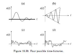
For responses (a) to (d) in Figure 10.30, explain why the response appears stable or unstable. x(t) (a) x(1) (b) x(t) My (c) (d) x(t) Figure 10.30: Four possible time-histories.
For the transfer function\[ \frac{\Theta_{o}(s)}{\Theta_{i}(s)}=\frac{K_{p}}{J s^{2}+K_{p}} \]solve for \(\theta_{o}(t)\) in terms of \(J, K_{p}\), and \(\theta_{i}(t)\). How do variations in the values of parameters \(J\) and \(K_{p}\) affect the behavior of \(\theta_{o}(t)\) ? Discuss and show
For a rotating element with \(P D\) controller, the transfer function is given by Equation 10.14, repeated here,\[ \frac{\Theta_{o}(s)}{\Theta_{i}(s)}=\frac{K_{p}\left(1+T_{d} s\right)}{J s^{2}+K_{p} T_{d} s+K_{p}} \]Explain how to select control parameters \(K_{p}\) and \(T_{d}\) that meet
A system transfer function is given by\[ T(s)=\frac{K s}{K s^{2}+1} \]Derive the sensitivity function and determine the value(s) of \(K\) that minimize sensitivity. Plot \(T(s)\) for \(K=1,10,100\) on one set of axes and draw conclusions from the comparison. Plot the sensitivity function for each
Repeat Problem 15 for the transfer function\[ T(s)=\frac{K s^{2}}{K s^{2}+s+1} \]Problem 15:A system transfer function is given by\[ T(s)=\frac{K s}{K s^{2}+1} \]Derive the sensitivity function and determine the value(s) of \(K\) that minimize sensitivity. Plot \(T(s)\) for \(K=1,10,100\) on
For the general transfer function\[ T(s)=\frac{C_{1}(s)+p C_{2}(s)}{C_{3}(s)+p C_{4}(s)+p^{2} C_{5}(s)} \]where \(C_{i}(s)\) are polynomials in \(s\), find the general sensitivity as a function of parameter \(p\).
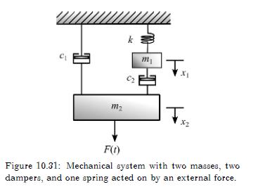
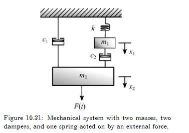
For the mechanical system shown in Figure 10.31, determine the differential equations of motion. Then, determine the state-space model where the input is the force and the output is the displacement of mass acted upon by the force. m k m F(t) Figure 10.31: Mechanical system with two masses, two
Calculate the transfer function of the linear system described by the following state and output equations,\[ \begin{aligned} \left\{\begin{array}{l} \dot{x}_{1}(t) \\ \dot{x}_{2}(t) \\ \dot{x}_{3}(t) \end{array}\right\} & =\left[\begin{array}{ccc} -2 & -5 & -4 \\ 1 & -1 & 0 \\ 0 & 1 & 0
Determine the transfer function of state and output equations in Example Problem 10.10 if \(\mathbf{A}, \mathbf{b}\), and \(\mathbf{c}\) are unchanged but \(D=1\). Is the transfer function proper, strictly proper, or not proper?
Determine the controllability and observability of the system\[ \begin{aligned} \left\{\begin{array}{l} \dot{x}_{1}(t) \\ \dot{x}_{2}(t) \end{array}\right\} & =\left[\begin{array}{cc} 0 & 1 \\ -2 & -3 \end{array}\right]\left\{\begin{array}{l} x_{1}(t) \\ x_{2}(t) \end{array}\right\} \\
Identify applications where a membrane model would apply.
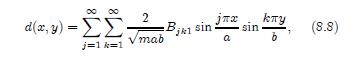
Derive Equation 8.8. 00 (2, 3) = 2 sin jk1 sin j=1 k=1 mab a (8.8) b
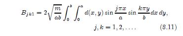
Derive Equation 8.11. Bjk1 = 2 ab d(x, y) sin a sin j, k = 1, 2,.... kxy dx dy, (8.11)
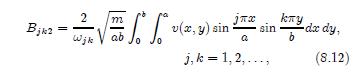
Derive Equation 8.12. Bjk2 - 2 Wijk ab a sin j, k = 1, 2,..., b -dx dy, (8.12)
Derive Equation 8.15. Explain the need for \(\theta=\) \(\theta_{0}+2 \pi j\). (R" + R'+3R) === (8.15) R R
Derive Bessel's equation and solve it in general.
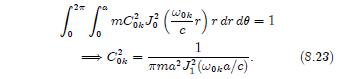
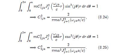
Derive Equations 8.23, 8.24, and 8.25. (Symbolic manipulation code such as Mathematica may be useful for the derivations.) Ok (wor) r dr de = 1 1 ma (wora/c) (8.23)
Derive by means of Hamilton's principle the differential equation of motion and the associated boundary conditions for a thin rectangular membrane. Give the physical interpretation of the boundary conditions.
Derive the frequency equation for a uniform annular membrane defined over the domain \(b \leq r \leq a\), with fixed boundaries at \(r=b\) and \(r=a\).
For the simply supported rectangular , suggest possible initial displacements \(d(x, y)\). Select one and solve for the complete solution. Assume zero initial velocity.
Find the response of a uniform rectangular membrane to the initial displacement\[ f(x, y)=\operatorname{Axy}(a-x)(b-y) \]with zero initial velocity.
Repeat Problem 10 for an assumed initial velocity \(v(x, y)\), with zero initial displacement.Problem 10:For the simply supported rectangular , suggest possible initial displacements \(d(x, y)\). Select one and solve for the complete solution. Assume zero initial velocity.
Convert the wave equation from Cartesian coordinates,\[ \frac{\partial^{2} u}{\partial t^{2}}=c^{2}\left(\frac{\partial^{2} u}{\partial x^{2}}+\frac{\partial^{2} u}{\partial y^{2}}\right) \]to polar coordinates,\[ \frac{\partial^{2} u}{\partial t^{2}}=c^{2}\left(\frac{\partial^{2} u}{\partial
Identify applications where a plate model would apply.
Derive by means of Hamilton's principle the equation of motion of a square plate.
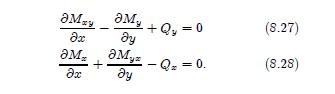
Derive Equations 8.27 and 8.28. +Qy=0 (8.27) x y Myz + - -Q== 0. (8.28)
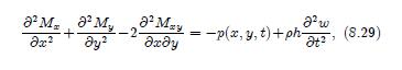
Derive Equation 8.29. + M M Mzy My -2- a w = -p(x, y, t)+ph (8.29) y 2 t
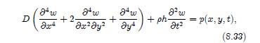
Derive Equation 8.33. (3+1+1)+ = p(x, y, t), (8.33)
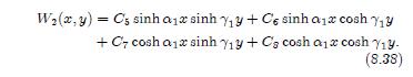
Derive Equation 8.38 Wz(2,3) = C, sinh an sinh Y13+Ca sinh an cosh 13 + C+ cosh ax sinh Yy + Cs cosh ax cosh Yy. (8.38)
Show that Equation 8.39 must be true for the given boundary conditions. = W(x, y) C sin ax sin yy. (8.39)
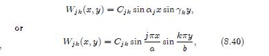
Derive coefficients\[ C_{j k}=\frac{2}{\sqrt{ho a b}} \]using the normalization procedure given for \(W_{j k}\) by Equation 8.40. == Wik(x, y) Cik sin aja sin Yky, or Wjk (x, y) =Cjk sin x : sin (8.40) a b
Derive the differential equation of motion for a nonuniform plate with varying thickness. Assume that the material properties such as Young's modulus and Poisson's ratio remain constant.
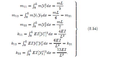
Derive Equations 8.54. m =mydx = = mL 5 mL = m12 myydx= m21 mamy dx = k11=EIYdx= 6 mL 7 (8.54) 4EI 6EI k12 = SEIYYdx= -k21 12EI k22=EIYdx
Show how the parameters \(k_{i j}\) and \(m_{i j}\) are derived.
Derive Rayleigh's quotient for a longitudinally vibrating beam.
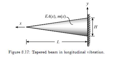
Estimate the fundamental frequency for the tapered beam of Figure 8.17 where\[ m(x)=m(1-x / L) \]and\[ E A(x)=E A(1-x / L) \]Compare your result to the exact value of \(\omega_{1}=\) \(2.40 \sqrt{E A / m L^{2}}\). X EA(x), m(x)- y H L Figure 8.17: Tapered beam in longitudinal vibration.
For Problem 26, estimate the first two natural frequencies using the Rayleigh-Ritz procedure. Assume a trial function of the form \(\mathcal{Y}(x)=c_{1} x^{2}+c_{2} x^{3}\). Compare the fundamental frequencies estimated by the Rayleigh-Ritz and the Rayleigh quotient methods.Problem 26:Estimate the
For the tapered beam sketched in Figure 8.17 undergoing transverse vibration, estimate the first two natural frequencies using the Rayleigh-Ritz procedure. Assume a trial function of the form \(\mathcal{Y}(x)=\) \(c_{1} x^{2}+c_{2} x^{3}\) and beam properties,\[ m(x)=ho A(x)=ho H(1-x / L) \]and\[
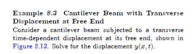
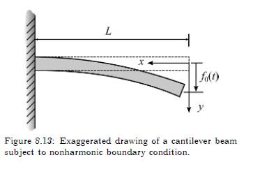
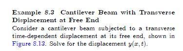
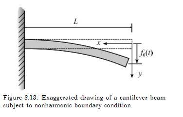
In Example 8.3, derive the general solution for \(f_{0}(t)=x \exp (-t / L)\). Example 8.3 Cantilever Beam with Transverse Displacement at Free End Consider a cantilever beam subjected to a transverse time-dependent displacement at its free end, shown in Figure 8.13. Solve for the displacement
Solve the problem of Example 8.3 where the only nonzero boundary condition is \(f_{1}(t)=\) \(\partial^{2} y(0, t) / \partial x^{2}\). Example 8.3 Cantilever Beam with Transverse Displacement at Free End Consider a cantilever beam subjected to a transverse time-dependent displacement at its free
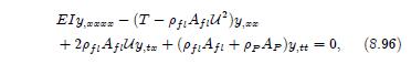
Derive Equation 8.96. Ely. (T-PAU),zz +2pfi Afilly to + (Pfi Afi + PPAP)y,tt = 0, (8.96)
Derive Equation 8.97. Ytt+2yt + (u - c)yxx = 0, (8.97)
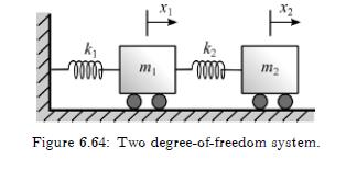
The two degree-of-freedom system in Figure 6.64 undergoes rectilinear motion. (a) Derive the flexibility influence coefficients. (b) Derive the stiffness influence coefficients. (c) Find the inverse of the flexibility matrix and show that this equals the stiffness matrix. (d) Write the matrix
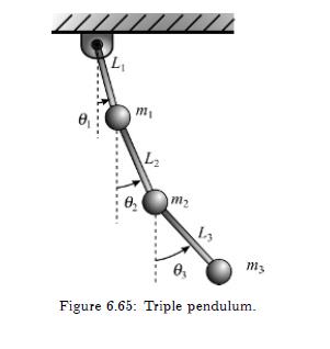
For the triple pendulum of Figure 6.65, determine the flexibility influence coefficients that relate the horizontal forces and the horizontal displacements. Find the inverse of the matrix of flexibility coefficients and then write the matrix equation of motion for this system. L L mz m3 Figure
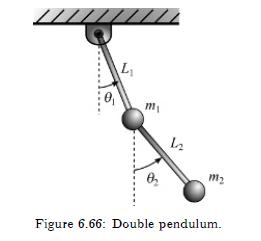
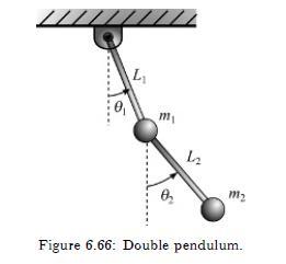
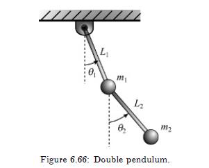
For the double pendulum of Figure 6.66, derive the equations of motion using (a) Newton's second law, and (b) Lagrange's equation. L 0 m m Figure 6.66: Double pendulum.
Derive the characteristic equation and the modal ratios for the system shown in Figure 6.66. L 0 m m Figure 6.66: Double pendulum.
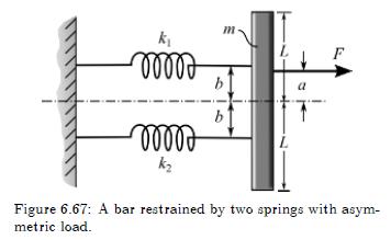
The system shown in Figure 6.67 consists of two linear springs with stiffnesses \(k_{1}\) and \(k_{2}\) and a uniform bar of mass \(m\) and length of \(2 L\). If the force \(F\) is acting at a distance \(a\) from the centerline as shown, derive Lagrange's equation of motion. Assume small motions. k
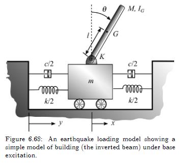
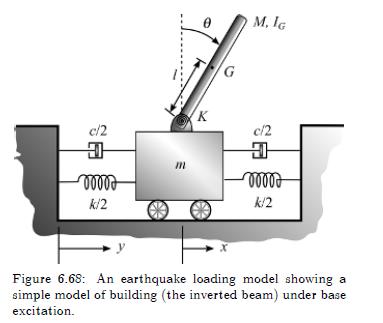
A simple lumped-parameter model of a building, shown as the inverted link in Figure 6.68, can be used for preliminary study of earthquake dynamics. Derive the equations of motion for this two degreeof-freedom system using (a) Newton's second law, and (b) Lagrange's equation. Let \(y(t)\) be the
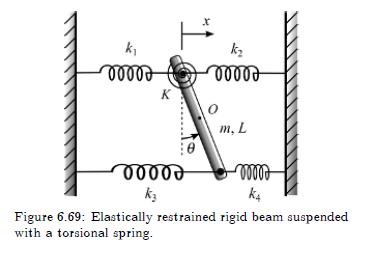
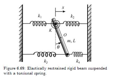
Derive the equation of motion for the elastically restrained rigid beam shown in Figure 6.69 using (a) Newton's second law, and (b) Lagrange's equation. k 00000 K k 00000 eeeee ? K3 m, L eelle K4 Figure 6.69: Elastically restrained rigid beam suspended with a torsional spring.
Use Hamilton's principle to derive the equations of motion for the structures shown in Figures (a) 6.66, (b) 6.68 , and (c) 6.69 . L m 12 m2 Figure 6.66: Double pendulum.
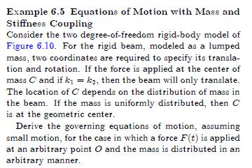
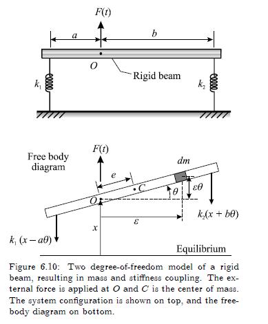
Derive the equations of motion for the problem of Example 6.5 using(a) Newton's second law,(b) Lagrange's equation, and(c) Hamilton's principle, and then solve for the response. Example 6.5 Equations of Motion with Mass and Stiffness Coupling Consider the two degree-of-freedom rigid-body model of
In Example 6.7 evaluate \(\bar{C}_{1}, \bar{C}_{2}, \phi_{1}\), and \(\phi_{2}\) using the given initial conditions: \(x_{1}(0)=1 \mathrm{~cm}, x_{2}(0)=\) \(-1 \mathrm{~cm}, \dot{x}_{1}(0)=3 \mathrm{~cm} / \mathrm{s}, \dot{x}_{2}(0)=-2 \mathrm{~cm} / \mathrm{s}\). Use \(\sqrt{k / m}=10
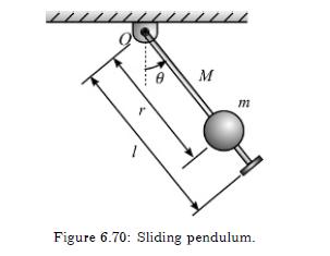
Consider the problem of the "sliding pendulum" drawn in Figure 6.70, where a mass slides along a frictionless rod which is assumed to be uniform and thin. Use (a) Newton's second law, and (b) Lagrange's equation to derive the equations of motion. Can the governing equations be linearized? Under
Linearize and solve the equations of motion derived in Problem 11. State all assumptions necessary for the linearization and explain them physically.Problem 11:Consider the problem of the "sliding pendulum" drawn in Figure 6.70, where a mass slides along a frictionless rod which is assumed to be
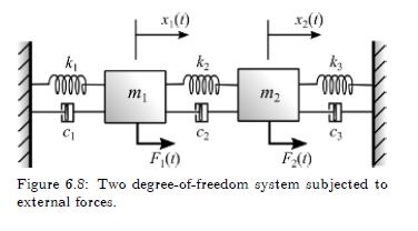
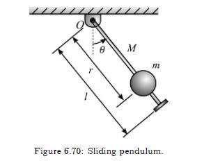
For the system shown in Figure 6.13, solve for the responses where \(k_{1}=k_{2}=k_{3}=k, m_{1}=m_{2}=\) \(m\), and where the initial conditions are \(x_{1}(0)=\) \(1, x_{2}(0)=1\), and zero initial velocities, all in appropriate units. Plot the modes, identifying the nodes. Plot \(\omega_{1,2}\)
Solve for the general response of the system given in Problem 1:\[ \begin{aligned} & {\left[\begin{array}{cc} m_{1} & 0 \\ 0 & m_{2} \end{array}\right]\left\{\begin{array}{c} \ddot{x}_{1} \\ \ddot{x}_{2} \end{array}\right\} } \\ + & {\left[\begin{array}{cc}
Solve for the general response of the system given in Problem 2 .Problem 2 :For the triple pendulum of Figure 6.65, determine the flexibility influence coefficients that relate the horizontal forces and the horizontal displacements. Find the inverse of the matrix of flexibility coefficients and
Linearize the governing equations of Problem 3 shown below and find the natural frequencies and mode shapes for \(m_{1}=m_{2}=m\) and \(l_{1}=l_{2}=l\). State all assumptions in the linearization process:\[ \begin{aligned} & \left(m_{1}+m_{2}\right) l_{1} \ddot{\theta}_{1}+m_{2}
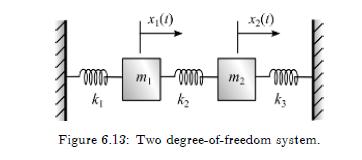
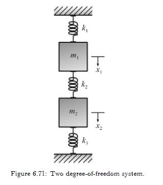
For the two degree-of-freedom system shown in Figure 6.71, determine the natural frequencies of oscillation about equilibrium and the respective modal ratios. Assume the following parameter values: \(m_{1}=10 \mathrm{~kg}, m_{2}=14 \mathrm{~kg}, k_{1}=4 \mathrm{~N} / \mathrm{m}, k_{2}=5\)
In Problem 6, using the governing equations of motion given below, assume a harmonic base motion and find the undamped response:\[ \begin{aligned} (m+M) \ddot{x}+M l\left(\ddot{\theta} \cos \theta-\dot{\theta}^{2} \sin \theta\right) & \\ -k(y-x)-c(\dot{y}-\dot{x}) & =0 \\ \left(I_{G}+M
Find the response of the freely vibrating system of Problem 7,\[ \begin{aligned} m(\ddot{x} & \left.+\frac{L}{2} \ddot{\theta}\right)+\left(k_{1}+k_{2}\right) x \\ & +\left(k_{3}+k_{4}\right)(x+L \theta)=0 \\ \frac{m L}{2} \ddot{x}+ & \left(I_{O}+m \frac{L}{2}\right)
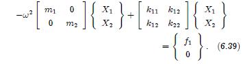
Suppose the system of Equation 6.38,\[ \begin{aligned} & {\left[\begin{array}{cc} m_{1} & 0 \\ 0 & m_{2} \end{array}\right]\left\{\begin{array}{l} \ddot{x}_{1} \\ \ddot{x}_{2} \end{array}\right\}} \\ & +\left[\begin{array}{cc} k_{11} & k_{12} \\ k_{21} & k_{22}
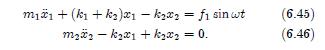
For the undamped vibration absorber problem governed by Equations 6.45 and 6.46,\[ \begin{aligned} m_{1} \ddot{x}_{1}+\left(k_{1}+k_{2}\right) x_{1}-k_{2} x_{2} & =f_{1} \sin \omega t \\ m_{2} \ddot{x}_{2}-k_{2} x_{1}+k_{2} x_{2} & =0 \end{aligned} \]assume that the absorber mass is also
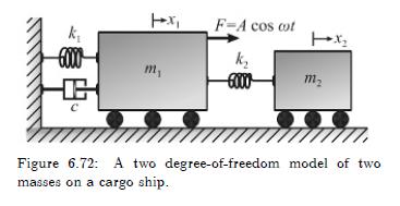
A cargo ship containing many boxes is at sea and experiences rough motion. Consider two masses in the cargo hold that are in close proximity when mass \(m_{1}\) is subjected to a force \(F=A \cos (\omega t+\phi)\) in line with the springs, as shown in Figure 6.72. The two masses are connected to
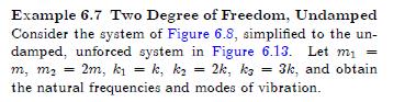
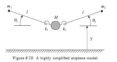
The vibration characteristics of an airplane are very complex due to its intricate system of structures and substructures. Suppose we consider the much simplified model of Figure 6.73, which is a three degree-of-freedom representation of the fuselage and wings. Derive the equations of motion using
What will change in our formulation and solution of Problem 23 if the symmetry assumption in the previous problem is removed? Discuss fully. Problem 23:The vibration characteristics of an airplane are very complex due to its intricate system of structures and substructures. Suppose we consider the
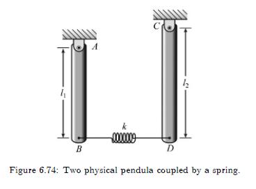
Two uniform rods \(A B\) and \(C D\) of linear density \(ho\) are suspended and connected by a spring as shown in Figure 6.74. The rods are in equilibrium when hanging in the vertical direction. (a) Derive the equations of motion of the system. (b) Find the natural frequencies of oscillation. (c)
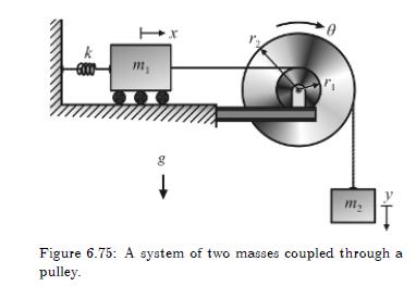
For the two degree-of-freedom system shown in Figure 6.75 derive the equations of motion. Assume that there is no slip between the cords that connect the masses to the pulley. The moment of inertia of the pulley about its point of rotation is \(I\). How would the formulation be different if
Complete the solution of Equation 6.55,\[ \begin{aligned} \left\{\begin{array}{l} \theta_{1}(t) \\ \theta_{2}(t) \end{array}\right\} & =C_{1}\left\{\begin{array}{c} 1 \\ 1 \end{array}\right\} \cos \left(\omega_{1} t-\phi_{1}\right) \\ & +C_{2}\left\{\begin{array}{c} 1 \\ -1 \end{array}\right\} \cos
Derive Equations 6.69 and 6.70,\[ \begin{aligned} x_{1}(t) & =e^{-a_{1} t}\left(r_{1} C_{1} \cos \omega_{d 1} t+r_{1}^{\prime} C_{2} \sin \omega_{d 1} t\right) \\ & +e^{-a_{2} t}\left(r_{2} C_{3} \cos \omega_{d 2} t+r_{2}^{\prime} C_{4} \sin \omega_{d 2} t\right) \\ x_{2}(t) & =e^{-a_{1}
Derive Equations 6.71 and 6.72,\[ \begin{aligned} x_{1}(t) & =B_{1}^{\prime} e^{-a_{1} t} \cos \left(\omega_{d 1} t-\phi_{d 1}^{\prime}\right) \\ & +B_{2}^{\prime} e^{-a_{2} t} \cos \left(\omega_{d 2} t-\phi_{d 2}^{\prime}\right) \\ x_{2}(t) & =B_{1} e^{-a_{1} t} \cos \left(\omega_{d 1}
Use the direct method to solve the equations of motion for a system with the following property matri- ces,\[ \begin{aligned} & {[M]=\left[\begin{array}{ll} 1 & 0 \\ 0 & 1 \end{array}\right], \quad[C]=\left[\begin{array}{cc} 5 & -2 \\ -2 & 5 \end{array}\right]} \\ &
Use the direct method to solve the equations of motion for a system with the following property matrices,\[ \begin{aligned} & {[M]=\left[\begin{array}{ll} 1 & 0 \\ 0 & 1 \end{array}\right], \quad[C]=\left[\begin{array}{cc} 2 & -1 \\ -1 & 1 \end{array}\right]} \\ &
Use the direct method to solve the equations of motion for a system with the following property matrices,\[ \begin{aligned} & {[M]=\left[\begin{array}{ll} 1 & 0 \\ 0 & 1 \end{array}\right], \quad[C]=\left[\begin{array}{cc} 5 & -2 \\ -2 & 3 \end{array}\right]} \\ &
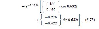
Derive Equation 6.78 showing all steps. +-0.115+ [{ 0.180 cos 0.632t 0.460 -0.276 -0.422 }. sin 0.632t (6.78)
Derive Equation 6.79. {u}[K]{u} = 0, (6.79)
Show that the orthogonality relations hold when there is coupling in both mass as well as in stiffness matrices as long as they are symmetric. This requires a derivation of the characteristic matrix and equation, the eigenvalues, and the eigenvectors.
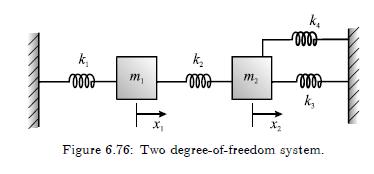
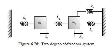
For the two degree-of-freedom system in Figure 6.76 undergoing longitudinal motion, derive the equations of motion utilizing each of the following approaches: (a) flexibility coefficients, (b) Newton's second law of motion, (c) Lagrange's equation, and (d) Hamilton's principle. Then, with the
In Problem 36, the system is forced with \(F_{1}(t)=\) \(A_{1} \cos \Omega_{1} t\) and \(F_{2}(t)=A_{2} \sin \Omega_{2} t\) acting on mass \(m_{1}\) and \(m_{2}\), respectively. Using modal analysis, solve for the forced response assuming initial conditions \(x_{1}(0)=0, \dot{x}_{1}(0)=v_{1},
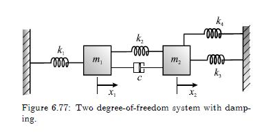
If Problem 36 is modified to include damping between the two masses as shown in Figure 6.77, solve for the case with no forcing using(a) modal analysis, and(b) the direct method.Problem 36:For the two degree-of-freedom system in Figure 6.76 undergoing longitudinal motion, derive the equations of
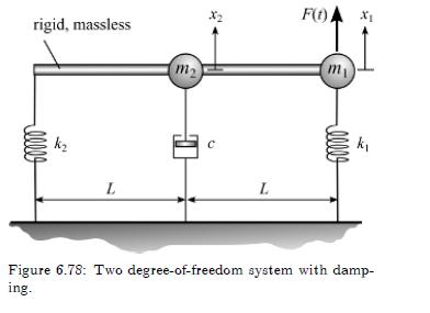
The two degree-of-freedom damped and forced system of Figure 6.78 oscillates about its equilibrium position. Use Lagrange's equation to formulate the problem and then solve the equations of motion for \(F(t)=A \cos \omega t\). Check whether proportional damping is a valid model here. If not, how
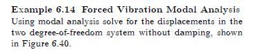
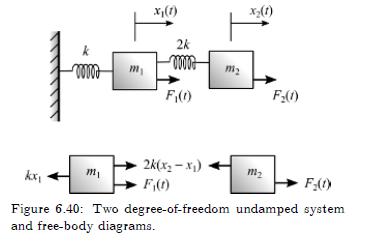
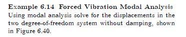
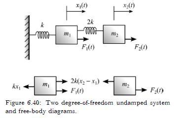
Solve Example 6.14 with the equation of motion\[ \begin{gathered} {\left[\begin{array}{cc} m & 0 \\ 0 & m \end{array}\right]\left\{\begin{array}{c} \ddot{x}_{1} \\ \ddot{x}_{2} \end{array}\right\}+\left[\begin{array}{cc} 3 k & -2 k \\ -2 k & 2 k
In Problem 40, solve the same equation of motion, except with \(F_{1}(t)=\cos (2 \sqrt{k / m} t)\) and \(F_{2}(t)=0\). Plot the displacement time histories.Problem 40:Solve Example 6.14 with the equation of motion\[\begin{gathered}{\left[\begin{array}{cc}m & 0 \\0 &
In Problem 40, solve for the response where the system damping is(a) \([C]=2[M]\),(b) \([C]=3[K]\),(c) \([C]=2[M]+3[K]\). In each discuss the results, especially regarding how the damping for each mode depends on the proportional damping model. Let \(\sqrt{k / m}\) be \(1 \mathrm{rad} /
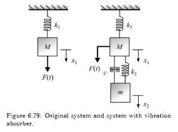
A vibrating mass is found to be oscillating with an amplitude that is too large. To reduce this amplitude, an auxiliary system is added as shown in Figure 6.79. This problem generally occurs when the forcing frequency is too close to the natural frequency of the primary system.The auxiliary system
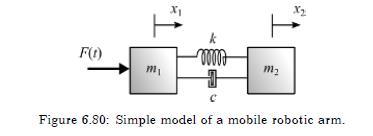
Figure 6.80 may be used as a simple model of a mobile robotic arm undergoing forced motion. The forcing is at the base of the arm. Derive the matrix equation of motion, and solve it in general for the response if(a) \(F(t)=u(t)\), and(b) \(F(t)=\cos 2 t\). Solve this problem in two ways: (i) using
The system shown in Figure 6.81 undergoes rotational motion. Derive the equations of motion and solve for the response in terms of the initial conditions, given by \(\theta_{1}(0), \dot{\theta}_{1}(0), \theta_{2}(0)\), and \(\dot{\theta}_{2}(0)\). Solve this problem in two ways: (a) using a
Two identical disks are connected by an elastic shaft of stiffness \(K\). The moment of inertia of each disk with respect to the axis of the shaft is \(J\). The system is at rest when a constant moment \(M\) is applied instantaneously to one of the disks. Determine the motion of the system assuming
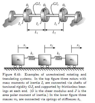
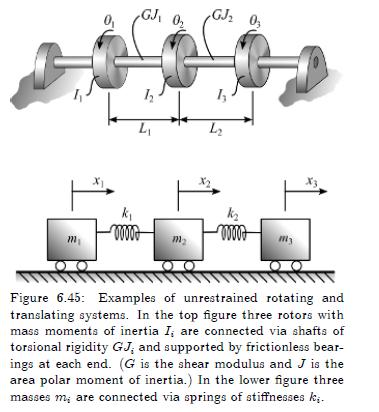
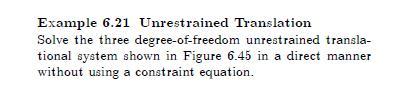
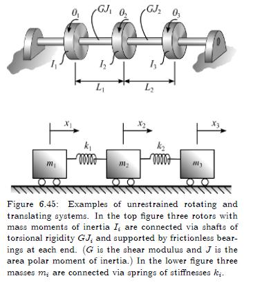
In Example 6.20, derive \([K]\). Example 6.20 Unrestrained Rotation Solve the three degree-of-freedom rotational model of Figure 6.45 and show how unrestrained rotation has ap- plications to rotating machinery.
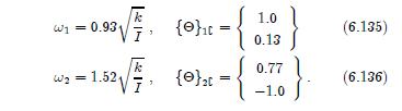
In Example 6.20, derive the eigenvalue problem for the constrained system and show that the frequencies and modes are given by Equations 6.135 and 6.136 . W =0.93 W1 == W = 1.52 k {0} = { 1.0 0.13 .} (6.135) {0} 20 = { 0.77 (6.136) -1.0
Solve Example 6.20, where \(k_{1}=3 \mathrm{~N}-\mathrm{m} / \mathrm{rad}, k_{2}=\) \(10 \mathrm{~N}-\mathrm{m} / \mathrm{rad}, I_{1}=5 \mathrm{~kg}-\mathrm{m}^{2} / \mathrm{rad}, I_{2}=2 I_{1}\), and \(I_{3}=\) \(I_{2} / 2\). Example 6.20 Unrestrained Rotation Solve the three degree-of-freedom
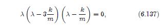
In Example 6.21, show how Equation 6.137 arises. (-) () = 0, (6.137)
For Example 6.21, show the steps in the derivation of the three modes of vibration. Example 6.21 Unrestrained Translation Solve the three degree-of-freedom unrestrained transla- tional system shown in Figure 6.45 in a direct manner without using a constraint equation.
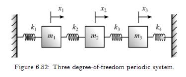
(a) For the three degree-of-freedom system shown in Figure 6.82, derive the equations of motion and solve for the frequencies and modes of vibration for the arbitrary stiffnesses \(k_{1}, k_{2}, k_{3}, k_{4}\) and masses \(m_{1}, m_{2}, m_{3}\). Then simplify these results for the case where all
In Problem 52, part (b), solve assuming \(k_{1}=k_{2}=\) \(k_{3}=k_{4}=k\) and \(m_{1}=m_{3}=m\) and \(m_{2}=m(1+\epsilon)\). Use the same parameter values. Discuss.Problem 52:(b) For the previous system, suppose that \(k_{1}=k_{3}=\) \(k_{4}=k=1 \mathrm{~N} / \mathrm{m}, m_{1}=m_{2}=m_{3}=m=1
Derive Equation 6.144. = k + k + 121 k kkz = (6.144) m2 m1m2
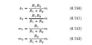
Derive Equations 6.150 to 6.153. RR k = -m2 (6.150) R + Ra RR3 k2 = R + R3 m (6.151) R m = -m (6.152) R + R3 Rs m2 = -m. (6.153) R+ R

Showing 100 - 200 of 2655

1
2
3
4
5
6
7
8
9
10
11
12
13
14
15
Last

Step by Step Answers

Services

Sitemap
Fun
Definitions
Become Tutor
Used Textbooks
Study Help Categories
Recent Questions
Expert Questions
Campus Wear
Sell Your Books

Company Info

Security
Copyrights
Privacy Policy
Terms & Conditions
SolutionInn Fee
Scholarship
Online Quiz
Give Feedback, Get Rewards

Get In Touch

About Us
Contact Us
Career
Jobs
FAQ
Student Discount
Campus Ambassador

Secure Payment

Download Our App

© 2026 SolutionInn. All Rights Reserved