New Semester
Started
Get
50% OFF
Study Help!
--h --m --s
Claim Now
Question Answers
Textbooks
Find textbooks, questions and answers
Oops, something went wrong!
Change your search query and then try again
S
Books
FREE
Study Help
Expert Questions
Accounting
General Management
Mathematics
Finance
Organizational Behaviour
Law
Physics
Operating System
Management Leadership
Sociology
Programming
Marketing
Database
Computer Network
Economics
Textbooks Solutions
Accounting
Managerial Accounting
Management Leadership
Cost Accounting
Statistics
Business Law
Corporate Finance
Finance
Economics
Auditing
Tutors
Online Tutors
Find a Tutor
Hire a Tutor
Become a Tutor
AI Tutor
AI Study Planner
NEW
Sell Books
Search
Search
Sign In
Register
study help
business
econometrics
Using Econometrics A Practical Guide 7th Edition A. H. Studenmund - Solutions
Between regressions (6.6.8) and (6.6.10), which model do you prefer? Why?
For the regression (6.6.8), test the hypothesis that the slope coefficient is not significantly different from 0.005.
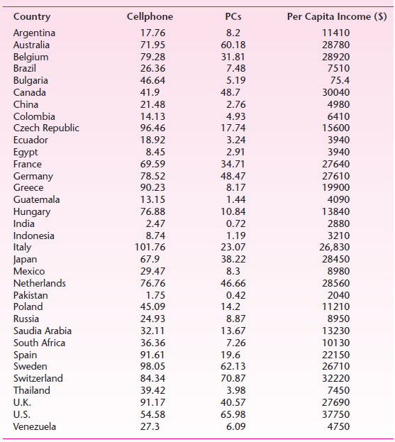
Refer to Example 3.3 in Chapter 3 to complete the following:In Example 3.3The following table gives data on the number of cell phone subscribers and the number of personal computers (PCs), both per 100 persons, and the purchasing power adjusted per capita income in dollars for a sample of 34
Consider the following model:Yi = eβ1+β2Xi / (1 + eβ1+β2Xi)As it stands, is this a linear regression model? If not, what “trick,” if any, can you use to make it a linear regression model? How would you interpret the resulting model? Under what circumstances might such a model be appropriate?
Repeat Exercise 6.20 but refer to the demand for personal computers given in the following equation. Is there a difference between the estimated income elasticities for cell phones and personal computers? If so, what factors might account for the difference?YÌ‚i = -6.5833 + 0.0018XiIn
Graph the following models (for ease of exposition, we have omitted the observation subscript, i):a. Y = β1Xβ2, for β2 > 1, β2 = 1, 0 < β2 < 1, …b. Y = β1eβ2X, for β2 > 0 and β2 < 0.Discuss where such models might be appropriate.
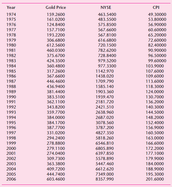
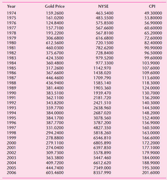
Refer to Problem 3.22.In exerciseTable 3.7 gives data on gold prices, the Consumer Price Index (CPI), and the New York Stock Exchange (NYSE) Index for the United States for the period 1974 €“2006. The NYSE Index includes most of the stocks listed on the NYSE, some 1500-plus.Table 3.7a.
Table 5.5 gives data on average public teacher pay (annual salary in dollars) and spending on public schools per pupil (dollars) in 1985 for 50 states and the District of Columbia.To find out if there is any relationship between teacher’s pay and per pupil expenditure in public schools, the
Consider the following regression output:Ŷi = 0.2033 + 0.6560Xtse = (0.0976) (0.1961)r2 = 0.397 RSS = 0.0544 ESS = 0.0358where Y = labor force participation rate (LFPR) of women in 1972 and X = LFPR of women in 1968. The regression results were obtained from a sample of 19 cities in the United
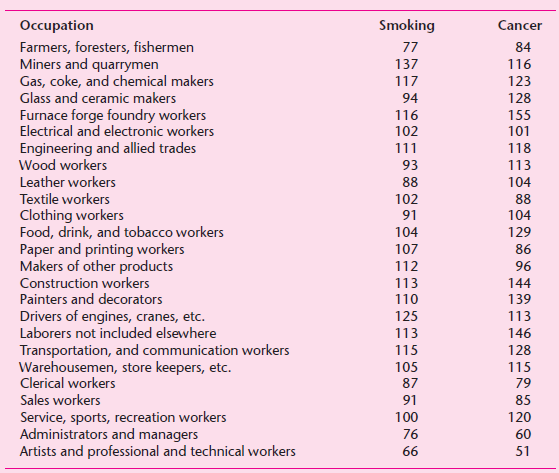
The following table provides data on the lung cancer mortality index (100 = average) and the smoking index (100 = average) for 25 occupational groups.a. Plot the cancer mortality index against the smoking index. What general pattern do you observe?b. Letting Y = cancer mortality index and X =
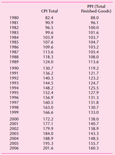
Following table gives annual data on the Consumer Price Index (CPI) and the Wholesale Price Index (WPI), also called Producer Price Index (PPI), for the U.S. economy for the period 1980€“2006.a. Plot the CPI on the vertical axis and the WPI on the horizontal axis. A priori, what kind of
R. A. Fisher has derived the sampling distribution of the correlation coefficient defined in Eq. (3.5.13).
Equation (5.3.5) can also be written asPr [β̂2 – 5α/2se(β̂2) < β2 < β̂2 + tα/2se (β̂2)] = 1 – αThat is, the weak inequality (≤) can be replaced by the strong inequality (<). Why?
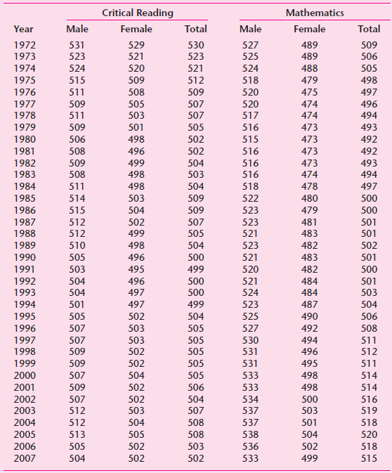
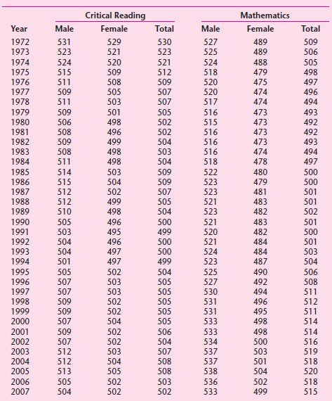
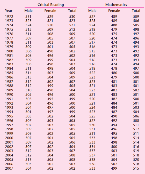
Repeat the exercise in the preceding problem but let Y and X denote the male and female critical reading scores, respectively.Repeat exerciseRefer to the SAT data given in Exercise 2.16.In exerciseThe following table gives data on mean Scholastic Aptitude Test (SAT) scores for collegebound seniors
Refer to the demand for cell phones regression given in Eq. (3.7.3).Eq (3.7.3)a. Is the estimated intercept coefficient significant at the 5 percent level of significance? What is the null hypothesis you are testing?b. Is the estimated slope coefficient significant at the 5 percent level? What is
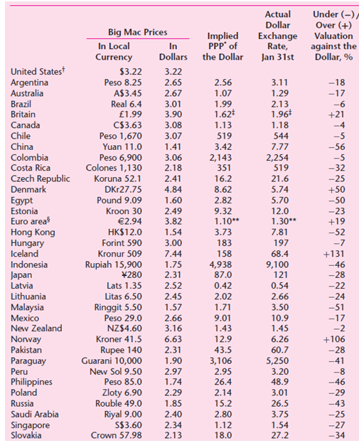
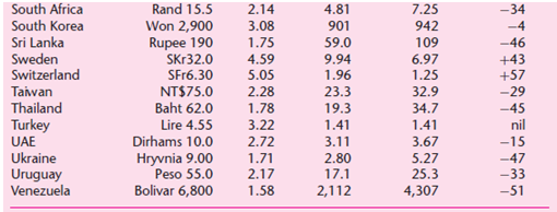
Since 1986 the Economist has been publishing the Big Mac Index as a crude, and hilarious, measure of whether international currencies are at their €œcorrect€ exchange rate, as judged by the theory of purchasing power parity (PPP). The PPP holds that a unit of currency should be
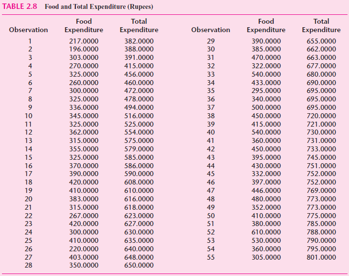
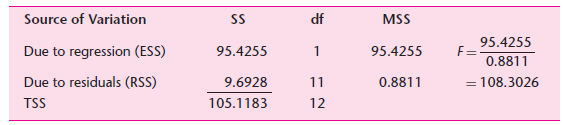
Set up the ANOVA table in the manner of Table 5.4 for the regression model given in Eq. (3.7.2) and test the hypothesis that there is no relationship between food expenditure and total expenditure in India.Table 5.4Eq (3.7.2) Source of Variation MSS df SS 95.4255 Due to regression (ESS) 95.4255 1
Suppose that the outcome of an experiment is classified as either a success or a failure. Letting X = 1 when the outcome is a success and X = 0 when it is a failure, the probability density, or mass, function of X is given byp(X = 0) = 1 − pp(X = 1) = p, 0 ≤ p ≤ 1What is the maximum
A random variable X follows the exponential distribution if it has the following probability density function (PDF):f(X) = (1/θ)e-X/θ for X > 0= 0
By applying the second-order conditions for optimization (i.e., second-derivative test), show that the ML estimators of β1, β2, and σ2obtained by solving Eqs. (9), (10), and (11) do in fact maximize the likelihood function in Eq. (4).Eq (9)Eq (10)Eq (11)Eq (4) Η
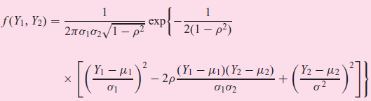
€œIf two random variables are statistically independent, the coefficient of correlation between the two is zero. But the converse is not necessarily true; that is, zero correlation does not imply statistical independence. However, if two variables are normally distributed, zero
Using the data given in Table 3.3, plot the number of cell phone subscribers against the number of personal computers in use. Is there any discernible relationship between the two? If so, how do you rationalize the relationship?
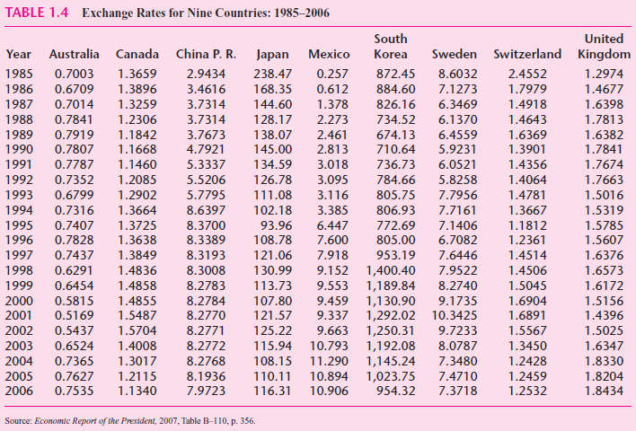
Table 1.4 gives the foreign exchange rates for nine industrialized countries for the years 1985€“2006. Except for the United Kingdom, the exchange rate is defined as the units of foreign currency for one U.S. dollar; for the United Kingdom, it is defined as the number of U.S. dollars for
Consider the following formulations of the two-variable PRF:Model I: Yi = β1 + β2Xi + uiModel II: Yi = α1 + α2(Xi – X̅ ) + uia. Find the estimators of β1 and α1. Are they identical? Are their variances identical?b. Find the estimators of β2 and α2. Are they identical? Are their
Suppose you run the following regression:Yi = β̂1 + β̂2xi +ûiwhere, as usual, yi and xi are deviations from their respective mean values.What will be the value of β̂1? Why? Will β̂2 be the same as that obtained from Eq. (3.1.6)? Why?
Let r1= coefficient of correlation between n pairs of values (Yi, Xi) and r2= coefficient of correlation between n pairs of values (aXi+ b, cYi+ d), where a, b, c, and d are constants. Show that r1= r2and hence establish the principle that the coefficient of correlation is invariant with respect to
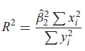
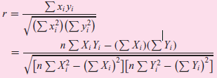
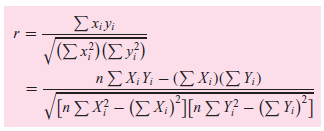
From a sample of 10 observations, the following results were obtained:ΣYi = 1,110 ΣXi = 1,700 ΣXiYi = 205,500ΣXi2 = 322,000 ΣYi2 = 132,100With coefficient of correlation r = 0.9758.
The following table gives data on gold prices, the Consumer Price Index (CPI), and the New York Stock Exchange (NYSE) Index for the United States for the period 1974 €“2006. The NYSE Index includes most of the stocks listed on the NYSE, some 1500-plus.a. Plot in the same scattergram gold
If X1, X2, and X3 are uncorrelated variables each having the same standard deviation, show that the coefficient of correlation between X1 + X2 and X2 + X3 is equal to 1/2. Why is the correlation coefficient not zero?
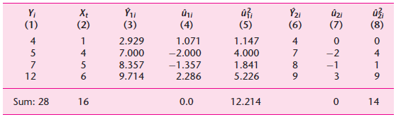
Show that the estimates β̂1= 1.572 and β̂2= 1.357 used in the first experiment of Table 3.1 are in fact the OLS estimators.Table 3.1 Y2i (6) Y; X¢ (2) ûi (4) ûzi (7) (3) 2.929 7.000 8.357 (5) 1.147 4.000 1.841 5.226 (8) (1) 4 1.071 4 4 5 -2.000
According to Malinvaud (see footnote 11), the assumption that E(ui | Xi) = 0 is quite important. To see this, consider the PRF: Y = β1 + β2Xi + ui . Now consider two situations:(i) β1 = 0, β2 = 1, and E(ui ) = 0;(ii) β1 = 1, β2 = 0, and E(ui ) = (Xi − 1).Now take the expectation of the PRF
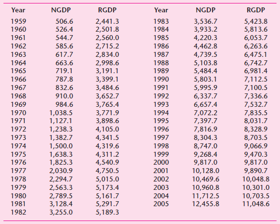
Table 3.8 gives data on gross domestic product (GDP) for the United States for the years 1959 2005.a. Plot the GDP data in current and constant (i.e., 2000) dollars against time.b. Letting Y denote GDP and X time (measured chronologically starting with 1 for 1959, 2 for 1960, through 47 for 2005),
Consider the sample regressionYi = β̂1 + β̂2Xi + ûiImposing the restrictions (i) Σûi = 0 and (ii) Σ ûiXi = 0, obtain the estimators β̂1 and β̂2 and show that they are identical with the least-squares estimators given in Eqs. (3.1.6) and (3.1.7). This method of obtaining
In the regression Yi = β1 + β2Xi + ui suppose we multiply each X value by a constant, say, 2. Will it change the residuals and fitted values of Y? Explain. What if we add a constant value, say, 2, to each X value?
Show that r2 defined in (3.5.5) ranges between 0 and 1. You may use the Cauchy–Schwarz inequality, which states that for any random variables X and Y the following relationship holds true:[E (XY)]2 ≤ E(X2) E(Y2)]
Let β̂YX and β̂XY represent the slopes in the regression of Y on X and X on Y, respectively. Show thatβ̂YX β̂XY = r2Where r is the coefficient of correlation between X and Y.
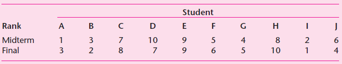
Spearman’s rank correlation coefficient rs is defined as follows:rs = 1 – 6 Σd2 / n(n2 – 1)Where d = difference in the ranks assigned to the same individual or phenomenon and n = number of individuals or phenomena ranked. Derive rs from r defined in Eq. (3.5.13). Rank the X and Y values from
Suppose in Exercise 3.6 that β̂YX β̂XY = 1. Does it matter then if we regress Y on X or X on Y? Explain carefully.
For the SAT example given in Exercise 2.16 do the following:In exerciseTable 2.9 gives data on mean Scholastic Aptitude Test (SAT) scores for collegebound seniors for 1972€“2007. These data represent the critical reading and mathematics test scores for both male and female students. The
Show that Eq. (3.5.14) in fact measures the coefficient of determination.Apply the definition of r given in Eq. (3.5.13) and recall that Σyiŷi = Σ(ŷi + ûi)ŷi = Σ ŷi2, and remember Eq.
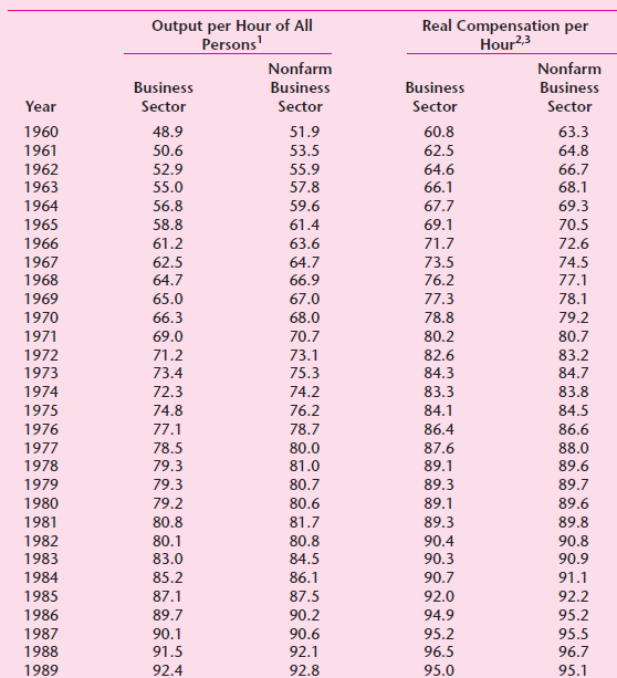
Table 3.6 gives data on indexes of output per hour (X) and real compensation per hour (Y) for the business and nonfarm business sectors of the U.S. economy for 1960€“2005. The base year of the indexes is 1992 = 100 and the indexes are seasonally adjusted.a. Plot Y against X for the two
The relationship between nominal exchange rate and relative prices. From annual observations from 1985 to 2005, the following regression results were obtained, where Y = exchange rate of the Canadian dollar to the U.S. dollar (CD/$) and X = ratio of the U.S. consumer price index to the Canadian
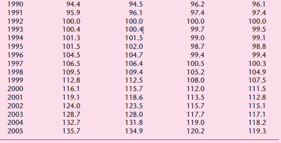
In Table 3.5, you are given the ranks of 10 students in midterm and final examinations in statistics. Compute Spearman€™s coefficient of rank correlation and interpret it. Student Rank E D н 4 5 3 2 9. 8 2 Midterm Final 10 3 5 9. 10
Regression without any regressor. Suppose you are given the model: Yi = β1 + ui.Use OLS to find the estimator of β1. What is its variance and the RSS? Does the estimated β1 make intuitive sense? Now consider the two-variable model Yi = β1 + β2Xi + ui . Is it worth adding Xi to the model? If
Explain with reason whether the following statements are true, false, or uncertain:a. Since the correlation between two variables, Y and X, can range from −1 to +1, this also means that cov (Y, X) also lies between these limits.b. If the correlation between two variables is zero, it means that
What is meant by an intrinsically linear regression model? If β2 in Exercise 2.7d were 0.8, would it be a linear or nonlinear regression model?
Are the following models linear regression models? Why or why not?a. Yi = eβ1 + β2Xi + uib. Yi = 1 / 1 + eβ1 + β2Xi + uic. ln Yi = β1 + β2 (1/Xi) + uid. Yi = β1 + (0.75-β1)e-β2(Xi-2) +uie. Yi = β1 + β32Xi + ui
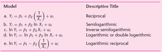
Determine whether the following models are linear in the parameters, or the variables, or both. Which of these models are linear regression models? Descriptive Title Model Reciprocal Semilogarithmic Inverse semilogarithmic Logarithmic or double logarithmic Logarithmic reciprocal a. Y; = B1 + B2 ( +
What do we mean by a linear regression model?
Why do we need regression analysis? Why not simply use the mean value of the regressand as its best value?
What is the role of the stochastic error term ui in regression analysis? What is the difference between the stochastic error term and the residual, ûi?
What is the difference between the population and sample regression functions? Is this a distinction without difference?
What is the conditional expectation function or the population regression function?
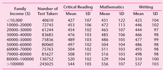
Table 2.10 presents data on mean SAT reasoning test scores classified by income for three kinds of tests: critical reading, mathematics, and writing. In Example 2.2, we presented Figure 2.7, which plotted mean math scores on mean family income.a. Refer to Figure 2.7 and prepare a similar graph
Table 2.9 gives data on mean Scholastic Aptitude Test (SAT) scores for collegebound seniors for 1972€“2007. These data represent the critical reading and mathematics test scores for both male and female students. The writing category was introduced in 2006. Therefore, these data are not
Table 2.8 gives data on expenditure on food and total expenditure, measured in rupees, for a sample of 55 rural households from India. (In early 2000, a U.S. dollar was about 40 Indian rupees.)a. Plot the data, using the vertical axis for expenditure on food and the horizontal axis for total
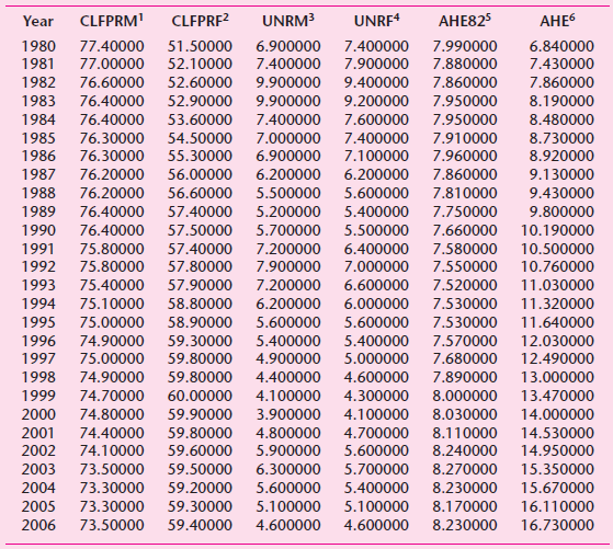
You are given the data in Table 2.7 for the United States for years 1980€“2006.a. Plot the male civilian labor force participation rate against male civilian unemployment rate. Eyeball a regression line through the scatter points. A priori, what is the expected relationship between the
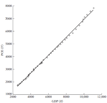
Is the regression line shown in Figure I.3 of the Introduction the PRF or the SRF? Why? How would you interpret the scatterpoints around the regression line? Besides GDP, what other factors, or variables, might determine personal consumption expenditure? 8000 7000 6000 5000 4000 3000 2000 1000 2000
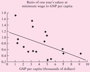
What does the scattergram in Figure 2.10 reveal? On the basis of this diagram, would you argue that minimum wage laws are good for economic well being? Ratio of one year's salary at minimum wage to GNP per capita 1.8 1.6 E 1.4 F 1.2 F 1.0 F 0.8 - 0.6 F 0.4 F 0.2 3 4 10 per capita (thousands of
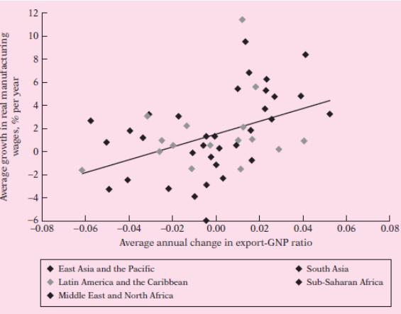
You are given the scattergram in Figure 2.8 along with the regression line. What general conclusion do you draw from this diagram? Is the regression line sketched in the diagram a population regression line or the sample regression line? 12 10 0.00 0.02 -0.08 -0.06 -0.04 -0.02 0.04 0.06 0.08
Consider the following nonstochastic models (i.e., models without the stochastic error term). Are they linear regression models? If not, is it possible, by suitable algebraic manipulations, to convert them into linear models?a. Yi = 1 / β1 + β2Xib. Yi = Xi / β1 + β2Xic. Yi = 1 / {1 + exp (-β1
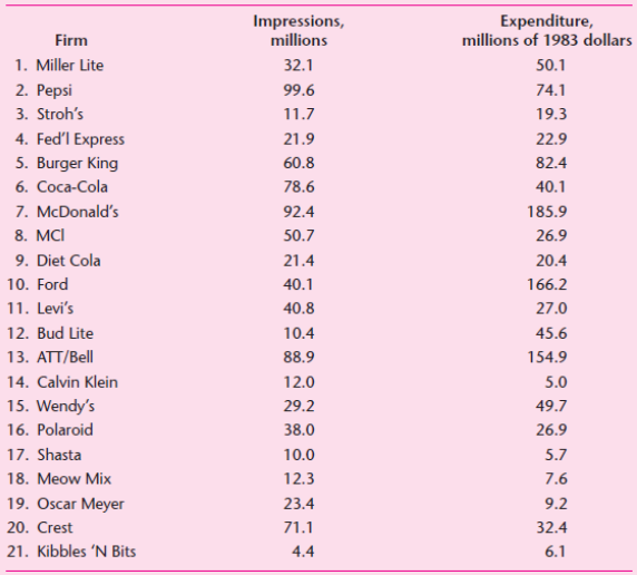
The data presented in Table 1.6 were published in the March 1, 1984, issue of The Wall Street Journal. They relate to the advertising budget (in millions of dollars) of 21 firms for 1983 and millions of impressions retained per week by the viewers of the products of these firms. The data are based
Controlled experiments in economics: On April 7, 2000, President Clinton signed into law a bill passed by both Houses of the U.S. Congress that lifted earnings limitations on Social Security recipients. Until then, recipients between the ages of 65 and 69 who earned more than $17,000 a year would
Suppose you were to develop an economic model of criminal activities, say, the hours spent in criminal activities (e.g., selling illegal drugs). What variables would you consider in developing such a model? See if your model matches the one developed by the Nobel laureate economist Gary
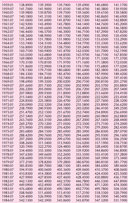
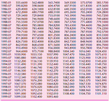
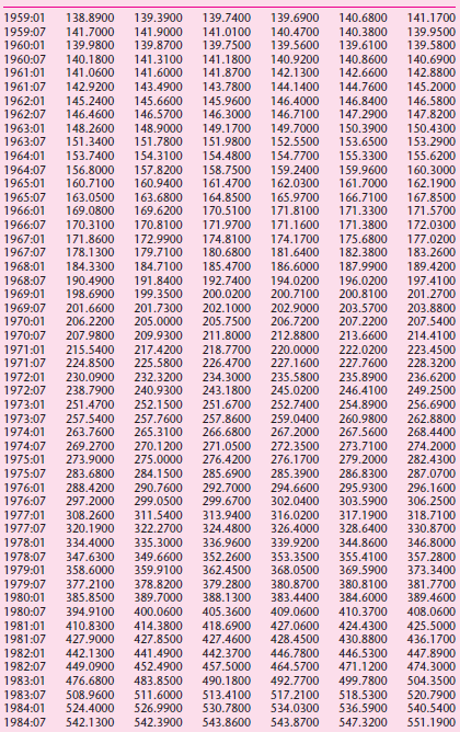
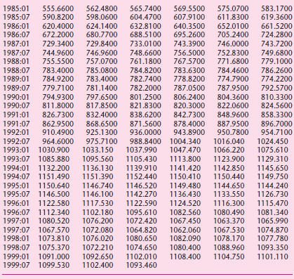
The data behind the M1 money supply in Figure 1.5 are given in Table 1.5. Can you give reasons why the money supply has been increasing over the time period shown in the table?Table 1.5 Seasonally adjusted M1 Supply: 1959:01-1999:07 (billions of dollars) 138.8900 139.3900 1959:01 139.7400 139.6900
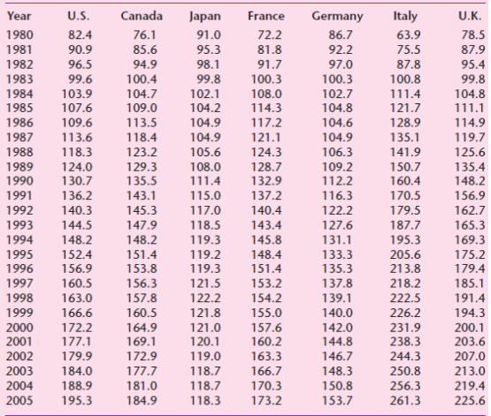
a. Using Table 1.3, plot the inflation rate of Canada, France, Germany, Italy, Japan, and the United Kingdom against the United States inflation rate.b. Comment generally about the behavior of the inflation rate in the six countries vis-Ã -vis the U.S. inflation rate.c. If you find that the
Table 1.3 gives data on the Consumer Price Index (CPI) for seven industrialized countries with 1982€“1984 = 100 as the base of the index.a. From the given data, compute the inflation rate for each country.b. Plot the inflation rate for each country against time (i.e., use the horizontal
Calculating VIFs typically involves running sets of auxiliary regressions, one regression for each independent variable in an equation. To get practice with this procedure, calculate the following:a. The VIFs for N, P, and I from the Woody’s data in Table 3.1b. The VIFs for BETA, EARN, and DIV
Simultaneous equations make sense in cross-sectional as well as time-series applications. For example, James Ragan examined the effects of unemployment insurance (hereafter UI) eligibility standards on unemployment rates and the rate at which workers quit their jobs. Ragan used a pooled data set
As an exercise to gain familiarity with the 2SLS program on your computer, take the data provided for the simple Keynesian model in Section 14.3, and:a. Estimate the investment function with OLS.b. Estimate the reduced form for Y with OLS.c. Substitute the Ŷ from your reduced form into the
The word recursive is used to describe an equation that has an impact on a simultaneous system without any feedback from the system to the equation. Which of the equations in the following systems are simultaneous, and which are recursive? Be sure to specify which variables are endogenous and which
In 2008, Goldman and Romley studied hospital demand by analyzing how 8,721 Medicare-covered pneumonia patients chose from among 117 hospitals in the greater Los Angeles area. The authors concluded that clinical quality (as measured by a low pneumonia mortality rate) played a smaller role in
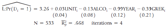
Because their college had just upgraded its residence halls, two seniors decided to build a model of the decision to live on campus. They collected data from 533 upper-class students (first-year students were required to live on campus) and estimated the following equation:Where:Di = 1 if the ith
In 2001, Heo and Tan published an article in which they used the Granger causality model to test the relationship between economic growth and democracy. For years, political scientists have noted a strong positive relationship between economic growth and democracy, but the authors of previous
Some farmers were interested in predicting inches of growth of corn as a function of rainfall on a monthly basis, so they collected data from the growing season and estimated an equation of the following form:Gt = β0 + β1Rt + β2Gt-1 + εtWhere:Gt = inches of growth of corn in month tRt = inches
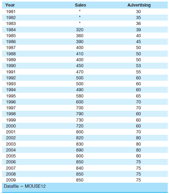
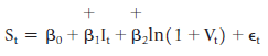
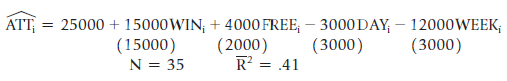
You€™ve been hired to determine the impact of advertising on gross sales revenue for €œFour Musketeers€ candy bars. Four Musketeers has the same price and more or less the same ingredients as competing candy bars, so it seems likely that only advertising affects
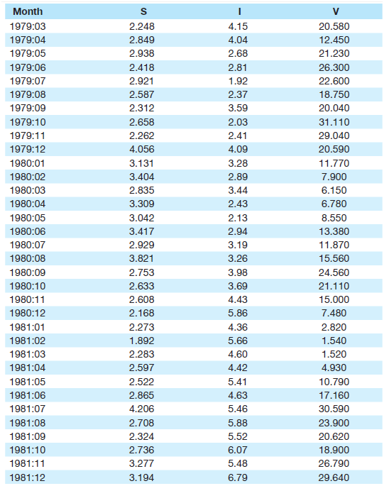
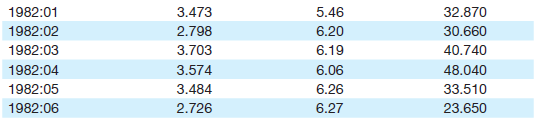
Let's investigate the possibility of heteroskedasticity in time-series data by looking at a model of the black market for U.S. dollars in Brazil that was studied by R. Dornbusch and C. Pechman. In particular, the authors wanted to know if the Demsetz-Bagehot bidask theory, previously tested on
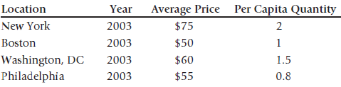
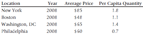
Suppose that you€™re interested in the effect of price on the demand for a €œsalon€ haircut and that you collect the following data for four U.S. cities for 2003:and for 2008:a. Estimate a cross-sectional OLS regression of per capita quantity as a function of average
The discussion of random assignment experiments in Section 16.1 includes models both with (Equation 16.2) and without (Equation 16.1) two additional observable factors (X1 and X2). In contrast, the discussion of natural experiments in Section 16.1 jumped immediately to Equation 16.3 below (which
James Stock and Mark Watson suggest a quite different approach to heteroskedasticity. They state that “economic theory rarely gives any reason to believe that the errors are homoskedastic. It therefore is prudent to assume that the errors might be heteroskedastic unless you have compelling
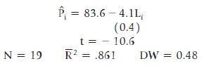
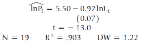
As an example of impure serial correlation caused by an incorrect functional form, let€™s return to the equation for the percentage of putts made (Pi) as a function of the length of the putt in feet (Li) that we discussed originally in Exercise 3 in Chapter 1. The complete documentation
Your friend is just finishing a study of attendance at Los Angeles Laker regular-season home basketball games when she hears that you€™ve read a chapter on serial correlation and asks your advice. Before running the equation on last season€™s data, she €œreviewed the
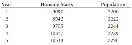
Recall from Section 9.5 that switching the order of a data set will not change its coefficient estimates. A revised order will change the Durbin€“Watson statistic, however. To see both these points, run regressions (HS = β0+ β1P + ε) and compare the
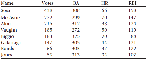
In 1998, Mark McGwire hit 70 homers to break Roger Maris€™s old record of 61, and yet McGwire wasn€™t voted the Most Valuable Player (MVP) in his league. To try to understand how this happened, you collect the following data on MVP votes, batting average (BA), home runs (HR),
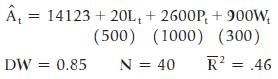
A researcher once attempted to estimate an asset demand equation that included the following three explanatory variables: current wealth Wt, wealth in the previous quarter Wt-1, and the change in wealth ΔWt = Wt - Wt-1. What problem did this researcher encounter? What should have been done to
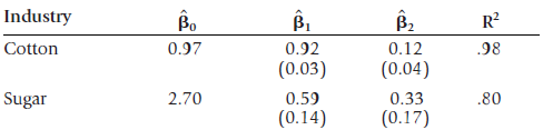
V. N. Murti and V. K. Sastri investigated the production characteristics of various Indian industries, including cotton and sugar. They specified Cobb–Douglas production functions for output (Q) as a double-log function of labor (L) and capital (K):lnQi = β0 + β1lnLi + β2lnKi +
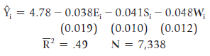
In an effort to explain regional wage differentials, you collect wage data from 7,338 unskilled workers, divide the country into four regions (Northeast, South, Midwest, and West), and estimate the following equation (standard errors in parentheses):Where:Yi = the hourly wage (in dollars) of the
Look over the following equations and decide whether they are linear in the variables, linear in the coefficients, both, or neither:a. Yi = β0 + β1X3i + εib. Yi = β0 + β1ln Xi + εic. ln Yi = β0 + β1ln Xi + εid. Yi = β0 + β1Xiβ2 + εie. Yiβ0 = β1 + β2X2i + εi
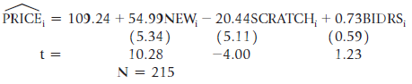
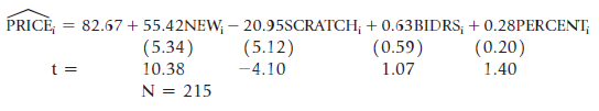
Let€™s return to the model of Exercises 3-7 and 5-8 of the auction price of iPods on eBay. In that model, we used datafile IPOD3 to estimate the following equation:Where:PRICEi = the price at which the ith iPod sold on eBayNEWi = a dummy variable equal to 1 if the ith iPod was new, 0
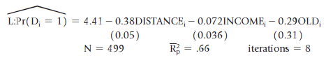
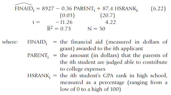
Let’s return to the model of financial aid awards at a liberal arts college that was first introduced in Section 2.2. In that section, we estimated the following equation (standard errors in parentheses):a. Create and test hypotheses for the coefficients of the independent variables.b. What
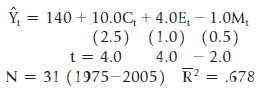
Consider the following annual model of the death rate (per million population) due to coronary heart disease in the United States (Yt):Where:Ct = per capita cigarette consumption (pounds of tobacco) in year tEt = per capita consumption of edible saturated fats (pounds of butter, margarine, and
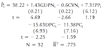
Frederick Schut and Peter VanBergeijk16 published an article in which they attempted to see if the pharmaceutical industry practiced international price discrimination by estimating a model of the prices of pharmaceuticals in a cross section of 32 countries. The authors felt that if price
Suppose that you€™ve been asked by the San Diego Padres baseball team to evaluate the economic impact of their new stadium by analyzing the team€™s attendance per game in the last year at their old stadium. After some research on the topic, you build the following model
Using the techniques of Section 5.3, test the following two-sided hypotheses:a. For Equation 5.8, test the hypothesis that:H0: 2 = 160.0HA: 2 ≠ 160.0at the 5-percent level of significance.b. For Equation 5.4, test the hypothesis that:H0: 3 = 0HA: 3 ≠ 0at the 1-percent level of
Create null and alternative hypotheses for the following coefficients:a. The impact of height on weightb. All the coefficients in Equation A in Exercise 5, Chapter 2c. All the coefficients in Y = β0 + β1X1 + β2X2 + β3X3 + ε, where Y is total gasoline used on a particular trip, X1 is miles
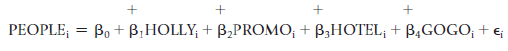
In Hollywood, most nightclubs hire €œpromoters,€ or people who walk around near the nightclub and try to convince passersby to enter the club. One of the nightclub owners asked a marketing consultant to estimate the effectiveness of such promoters in terms of their ability to
Which of the following pairs of independent variables would violate Assumption VI? (That is, which pairs of variables are perfect linear functions of each other?)a. Right shoe size and left shoe size (of students in your class)b. Consumption and disposable income (in the United States over the last
Let’s get some more experience with the six steps in applied regression. Suppose that you’re interested in buying an Apple iPod (either new or used) on eBay (the auction website) but you want to avoid overbidding. One way to get an insight into how much to bid would be to run a regression on
The Graduate Record Examination (GRE) subject test in economics was a multiple-choice measure of knowledge and analytical ability in economics that was used mainly as an entrance criterion for students applying to Ph.D. programs in the “dismal science.” For years, critics claimed that the GRE,
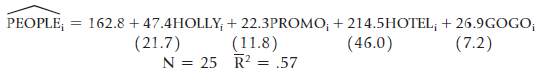
Do liberal arts colleges pay economists more than they pay other professors? To find out, we looked at a sample of 2,929 small-college faculty members and built a model of their salaries that included a number of variables, four of which were:Where:Si = the salary of the ith college professorMi = a
Showing 4000 - 4100
of 4105
First
28
29
30
31
32
33
34
35
36
37
38
39
40
41
42
Step by Step Answers

![Σxy / (Σx?) (ΣΥ?) η ΣΧΥ-(ΣΧ)(Σ Υ) [μΣΧ - (ΣΧ);]μ ΣΥ - (Σ] || ||](https://dsd5zvtm8ll6.cloudfront.net/si.question.images/images/question_images/1521/6/3/5/7075ab2517b129fcblob)