New Semester
Started
Get
50% OFF
Study Help!
--h --m --s
Claim Now
Question Answers
Textbooks
Find textbooks, questions and answers
Oops, something went wrong!
Change your search query and then try again
S
Books
FREE
Study Help
Expert Questions
Accounting
General Management
Mathematics
Finance
Organizational Behaviour
Law
Physics
Operating System
Management Leadership
Sociology
Programming
Marketing
Database
Computer Network
Economics
Textbooks Solutions
Accounting
Managerial Accounting
Management Leadership
Cost Accounting
Statistics
Business Law
Corporate Finance
Finance
Economics
Auditing
Tutors
Online Tutors
Find a Tutor
Hire a Tutor
Become a Tutor
AI Tutor
AI Study Planner
NEW
Sell Books
Search
Search
Sign In
Register
study help
business
introduction to probability statistics
Probability And Statistics For Engineers 9th Global Edition Richard Johnson, Irwin Miller, John Freund - Solutions
The freshness of produce at a mega-store is rated a scale of 1 to 5 , with 5 being very fresh. From a random sample of 36 customers, the average score was 3.5 with a standard deviation of 0.8.(a) Obtain a \(90 \%\) confidence interval for the population mean, \(\mu\), or the mean score for all
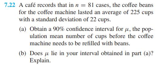
A café records that in \(n=81\) cases, the coffee beans for the coffee machine lasted an average of 225 cups with a standard deviation of 22 cups.(a) Obtain a 90\% confidence interval for \(\mu\), the population mean number of cups before the coffee machine needs to be refilled with beans.(b) Does
In an air-pollution study performed at an experiment station, the following amount of suspended benzenesoluble organic matter (in micrograms per cubic meter) was obtained for eight different samples of air:\[\begin{array}{llllllll}2.2 & 1.8 & 3.1 & 2.0 & 2.4 & 2.0 & 2.1 & 1.2\end{array}\]Assuming
Modify the formula for \(E\) on page 216 so that it applies to large samples which constitute substantial portions of finite populations, and use the resulting formula for the following problems:(a) A sample of 50 scores on the admission test for a school of engineering is drawn at random from the
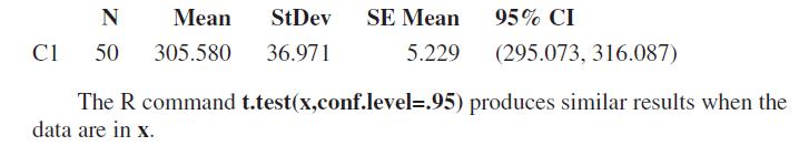
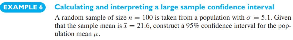
Instead of the large sample confidence interval formula for \(\mu\) on page 230, we could have given the alternative formula\[\bar{x}-z_{\alpha / 3} \cdot \frac{\sigma}{\sqrt{n}}Explain why the one on page 230 is narrower, and hence preferable, to the one given here. EXAMPLE 6 Calculating and
Suppose that we observe a random variable having the binomial distribution. Let \(X\) be the number of successes in \(n\) trials.(a) Show that \(\frac{X}{n}\) is an unbiased estimate of the binomial parameter \(p\).(b) Show that \(\frac{X+1}{n+2}\) is not an unbiased estimate of binomial parameter
The statistical program MINITAB will calculate the small sample confidence interval for \(\mu\). With the nanopillar height data in \(\mathrm{C} 1\),produces the output(a) Obtain a \(90 \%\) confidence interval for \(\mu\).(b) Obtain a 95\% confidence interval for \(\mu\) with the aluminum alloy
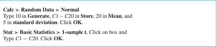
You can simulate the coverage of the small sample confidence intervals for \(\mu\) by generating 20 samples of size 10 from a normal distribution with \(\mu=20\) and \(\sigma=5\) and computing the \(95 \%\) confidence intervals according to the formula on page 231.Using MINITAB:(a) From your
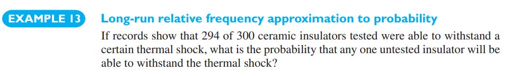
Refer to Example 13, Chapter 3, where 294 out of 300 ceramic insulators were able to survive a thermal shock.(a) Obtain the maximum likelihood estimate of the probability that a ceramic insulator will survive a thermal shock.(b) Suppose a device contains 3 ceramic insulators and all must survive
Refer to Example 7, Chapter 10, where 48 of 60 transceivers passed inspection.(a) Obtain the maximum likelihood estimate of the probability that a transceiver will pass inspection.(b) Obtain the maximum likelihood estimate that the next two transceivers tested will pass inspection.Data From Example
The daily number of accidental disconnects with a server follows a Poisson distribution. On five days\[\begin{array}{lllll}2 & 5 & 3 & 3 & 7\end{array}\]accidental disconnects are observed.(a) Obtain the maximum likelihood estimate of \(\lambda\).(b) Find the maximum likelihood estimate of the
In one area along the interstate, the number of dropped wireless phone connections per call follows a Poisson distribution. From four calls, the number of dropped connections is\[\begin{array}{llll}2 & 0 & 3 & 1\end{array}\](a) Find the maximum likelihood estimate of \(\lambda\).(b) Obtain the
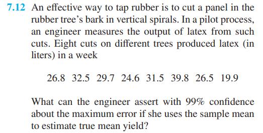
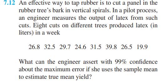
Refer to Exercise 7.12.(a) Obtain the maximum likelihood estimates of \(\mu\) and \(\sigma\).(b) Find the maximum likelihood of the probability that the next run will have a production greater than 38 liters.Data From Exercise 7.12 7.12 An effective way to tap rubber is to cut a panel in the rubber
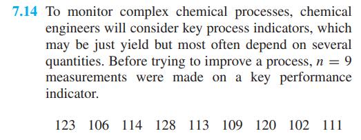
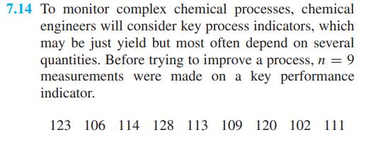
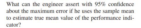
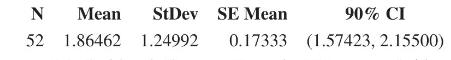
Refer to Exercise 7.14.(a) Obtain the maximum likelihood estimates of \(\mu\) and \(\sigma\).(b) Find the maximum likelihood of the coefficient of variation \(\sigma / \mu\).Data From Exercises 7.14What can the engineer assert with 95% confidence about the maximum error if he uses the sample mean
Find the maximum likelihood estimator of \(p\) when\[f(x ; p)=p^{x}(1-p)^{1-x} \quad \text { for } \quad x=0,1\]
Let \(x_{1}, \ldots, x_{n}\) be the observed values of a random sample of size \(n\) from the exponential distribution \(f(x ; \beta)=\beta^{-1} e^{-x / \beta}\) for \(x>0\).(a) Find the maximum likelihood estimator of \(\beta\).(b) Obtain the maximum likelihood estimator of the probability that
Let \(X\) have the negative binomial distribution\(f(x)=\left(\begin{array}{l}x-1 \\ r-1\end{array}\right) p^{r}(1-p)^{x-r}\) for \(x=r, r+1, \ldots\)(a) Obtain the maximum likelihood estimator of \(p\).(b) For one engineering application, it is best to use components with a superior finish.
A civil engineer wants to establish that the average time to construct a new two-storey building is less than 6 months.(a) Formulate the null and alternative hypotheses.(b) What error could be made if \(\mu=6\) ? Explain in the context of the problem.(c) What error could be made if \(\mu=5.5\) ?
A manufacturer of four-speed clutches for automobiles claims that the clutch will not fail until after 50,000 miles.(a) Interpreting this as a statement about the mean, formulate a null and alternative hypothesis for verifying the claim.(b) If the true mean is 55,000 miles, what error can be made?
An airline claims that the typical flying time between two cities is 56 minutes.(a) Formulate a test of hypotheses with the intent of establishing that the population mean flying time is different from the published time of 56 minutes.(b) If the true mean is 50 minutes, what error can be made?
A manufacturer wants to establish that the mean life of a gear when used in a crusher is over 55 days. The data will consist of how long gears in 80 different crushers have lasted.(a) Formulate the null and alternative hypotheses.(b) If the true mean is 55 days, what error could be made? Explain
A statistical test of hypotheses includes the step of setting a maximum for the probability of falsely rejecting the null hypothesis. Engineers make many measurements on critical bridge components to decide if a bridge is safe or unsafe.(a) Explain how you would formulate the null hypothesis.(b)
Suppose you are scheduled to ride a space vehicle that will orbit the earth and return. A statistical test of hypotheses includes the step of setting a maximum for the probability of falsely rejecting the null hypothesis. Engineers need to make various measurements to decide if it is safe or unsafe
Suppose that an engineering firm is asked to check the safety of a dam. What type of error would it commit if it erroneously rejects the null hypothesis that the dam is safe? What type of error would it commit if it erroneously fails to reject the null hypothesis that the dam is safe? Would would
Suppose that we want to test the null hypothesis that an antipollution device for cars is effective. Explain under what conditions we would commit a Type I error and under what conditions we would commit a Type II error.
If the criterion on page 242 is modified so that the manufacturer's claim is accepted for \(\bar{X}>1640\) cycles, find(a) the probability of a Type I error;(b) the probability of a Type II error when \(\mu=1680\) cycles. EXAMPLE 16 Not all samples will lead to a correct assessment of water
Suppose that in the electric car battery example on page 242, \(n\) is changed from 36 to 50 while everything else remains the same. Find(a) the probability of a Type I error;(b) the probability of a Type II error when \(\mu=1680\) cycles. EXAMPLE 16 Tests of Hypotheses There are many problems in
It is desired to test the null hypothesis \(\mu=30\) minutes against the alternative hypothesis \(\mu
Several square inches of gold leaf are required in the manufacture of a high-end component. Suppose that, the population of the amount of gold leaf has \(\sigma=8.4\) square inches. We want to test the null hypothesis \(\mu=80.0\) square inches against the alternative hypothesis \(\mu
A producer of extruded plastic products finds that his mean daily inventory is 1,250 pieces. A new marketing policy has been put into effect and it is desired to test the null hypothesis that the mean daily inventory is still the same. What alternative hypothesis should be used if(a) it is desired
Specify the null and alternative hypotheses in each of the following cases.(a) A car manufacturer wants to establish the fact that in case of an accident, the installed safety gadgets saved the lives of the passengers in more than \(90 \%\) of accidents.(b) An electrical engineer wants to establish
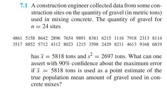
Refer to Exercise 7.1 where a construction engineer recorded the quantity of gravel (in metric tons) used in concrete mixes. The quantity of gravel for \(n=24\) sites has \(\bar{x}=5,818\) tons and \(s^{2}=7,273,809\) so \(s=\) 2,697 tons.(a) Construct a test of hypotheses with the intent of
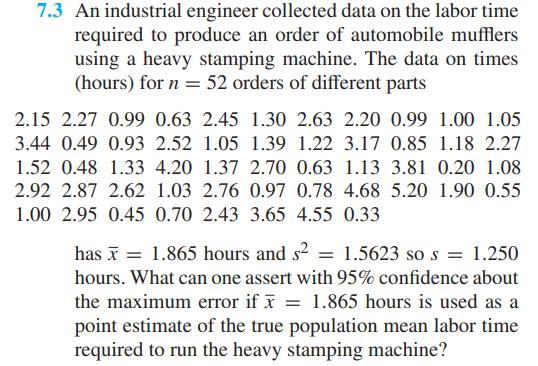
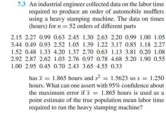
Refer to data in Exercise 7.3 on the labor time required to produce an order of automobile mufflers using a heavy stamping machine. The times (hours) for \(n=52\) orders of different parts has \(\bar{x}=1.865\) hours and \(s^{2}=1.5623\), so \(s=1.250\) hours.(a) Conduct a test of hypotheses with
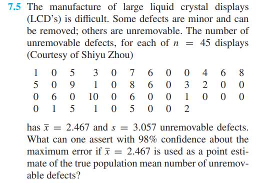
Refer to Exercise 7.5, where the number of unremovable defects, for each of \(n=45\) displays, has \(\bar{x}=\) 2.467 and \(s=3.057\) unremovable defects.(a) Conduct a test of hypotheses with the intent of showing that the mean number of unremovable defects is less than 3.6. Take
Refer to Exercise 7.12, where, in a pilot process, vertical spirals were cut to produce latex from \(n=8\) trees to yield (in liters) in a week.26.8 32.5 29.7 24.6 31.5 39.8 26.5 19.9(a) Conduct a test of hypotheses with the intent of showing that the mean
Refer to Exercise 7.14, where \(n=9\) measurements were made on a key performance indicator.\[\begin{array}{lllllllll}123 & 106 & 114 & 128 & 113 & 109 & 120 & 102 & 111\end{array}\](a) Conduct a test of hypotheses with the intent of showing that the mean key
Refer to Exercise 7.22, where, in \(n=81\) cases, the coffee machine needed to be refilled with beans after 225 cups with a standard deviation of 22 cups.(a) Conduct a test of hypotheses with the intent of showing that the mean number of cups is greater than 218 cups. Take \(\alpha=0.01\).(b) Based
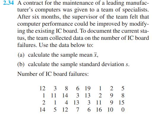
Refer to Exercise 2.34, page 46, concerning the number of board failures for \(n=32\) integrated circuits. A computer calculation gives \(\bar{x}=7.6563\) and \(s=\) 5.2216. At the 0.01 level of significance, conduct a test of hypotheses with the intent of showing that the mean is greater than 7
In 64 randomly selected hours of production, the mean and the standard deviation of the number of acceptable pieces produced by a automatic stamping machine are \(\bar{x}=1,038\) and \(s=146\). At the 0.05 level of significance, does this enable us to reject the null hypothesis \(\mu=1,000\)
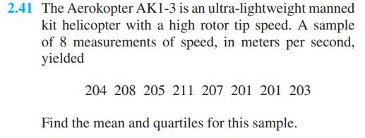
With reference to the thickness measurements in Exercise 2.41 , test the null hypothesis that \(\mu=30.0\) versus a two-sided alternative. Take \(\alpha=0.05\).Data From Exercise 2.41 2.41 The Aerokopter AK1-3 is an ultra-lightweight manned kit helicopter with a high rotor tip speed. A sample of 8
A random sample of 6 steel beams has a mean compressive strength of 58,392 psi (pounds per square inch) with a standard deviation of 648 psi. Use this information and the level of significance \(\alpha=0.05\) to test whether the true average compressive strength of the steel from which this sample
A manufacturer claims that the average tar content of a certain kind of cigarette is \(\mu=14.0\). In an attempt to show that it differs from this value, five measurements are made of the tar content ( \(\mathrm{mg}\) per cigarette):\[\begin{array}{lllll}14.5 & 14.2 & 14.4 & 14.3 &
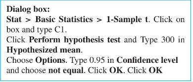
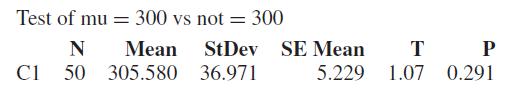
The statistical program MINITAB will calculate \(t\) tests. With the nanopillar height data in \(\mathrm{C} 1\),You must compare your preselected \(\alpha\) with the printed \(P\)-value in order to obtain the conclusion of your test. To perform a \(Z\) test, you need to find the \(P\)-value
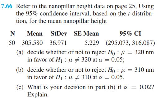
Refer to the nanopillar height data on page 25. Using the \(95 \%\) confidence interval, based on the \(t\) distribution, for the mean nanopillar height(a) decide whether or not to reject \(H_{0}: \mu=320 \mathrm{~nm}\) in favor of \(H_{1}: \mu eq 320\) at \(\alpha=0.05\);(b) decide whether or not
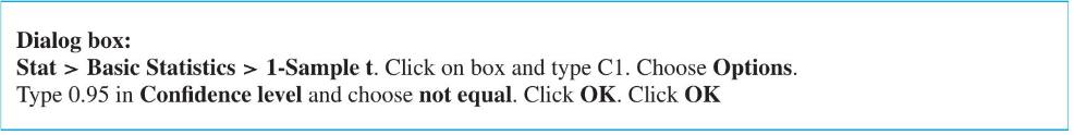
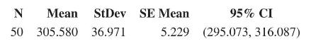
Repeat Exercise 7.66 but replace the \(t\) test with the large sample \(Z\) test.Data From Exercise 7.66 7.66 Refer to the nanopillar height data on page 25. Using the 95% confidence interval, based on the t distribu- tion, for the mean nanopillar height N Mean StDev SE Mean 50 305.580 36.971
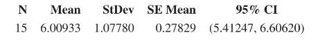
Refer to the green gas data on page 241 . Using the \(95 \%\) confidence interval, based on the \(t\) distribution for the mean yield(a) decide whether or not to reject \(H_{0}: \mu=5.5 \mathrm{gal}\) in favor of \(H_{0}: \mu eq 5.5\) at \(\alpha=0.05\);(b) decide whether or not to reject \(H_{0}:
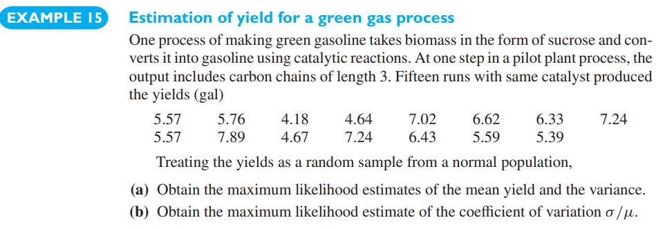
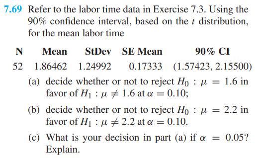
Refer to the labor time data in Exercise 7.3. Using the \(90 \%\) confidence interval, based on the \(t\) distribution, for the mean labor time(a) decide whether or not to reject \(H_{0}: \mu=1.6\) in favor of \(H_{1}: \mu eq 1.6\) at \(\alpha=0.10\);(b) decide whether or not to reject \(H_{0}:
Repeat Exercise 7.69 but replace the \(t\) test with the large sample \(Z\) test.Data From Exercise 7.69 7.69 Refer to the labor time data in Exercise 7.3. Using the 90% confidence interval, based on the t distribution, for the mean labor time N Mean 52 1.86462 StDev 1.24992 SE Mean 0.17333 90%
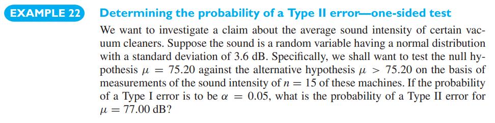
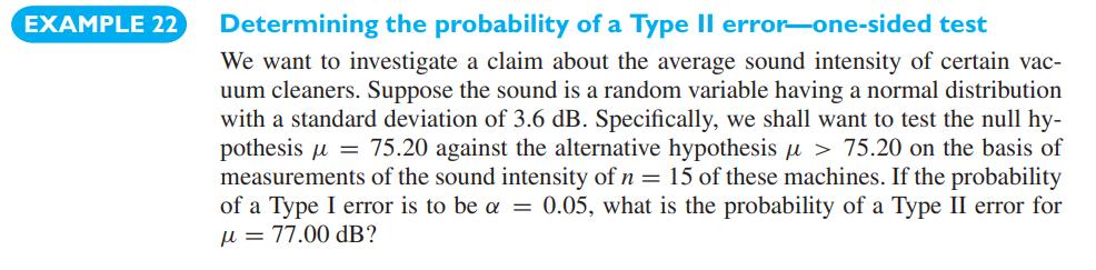
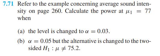
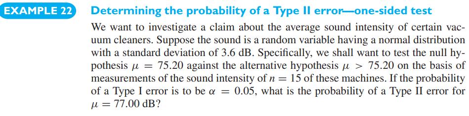
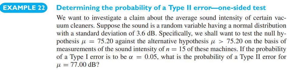
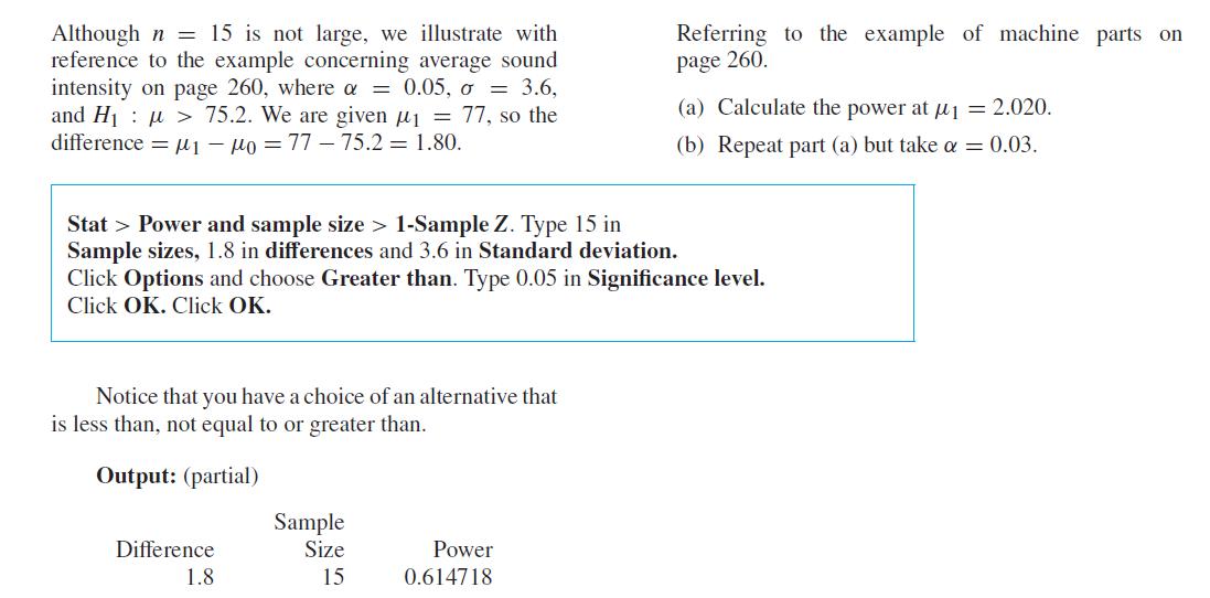
Refer to the example concerning average sound intensity on page 260 . Calculate the power at \(\mu_{1}=77\) when(a) the level is changed to \(\alpha=0.03\).(b) \(\alpha=0.05\) but the alternative is changed to the twosided \(H_{1}: \mu eq 75.2\). EXAMPLE 22 Determining the probability of a Type II
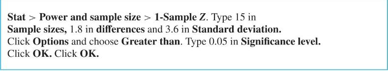
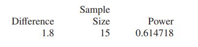
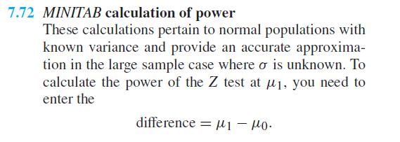
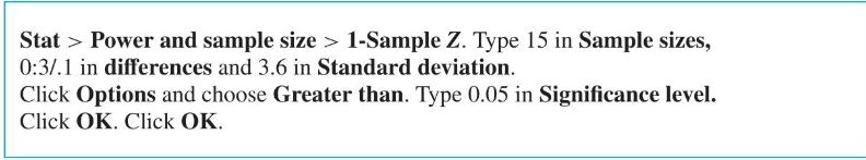
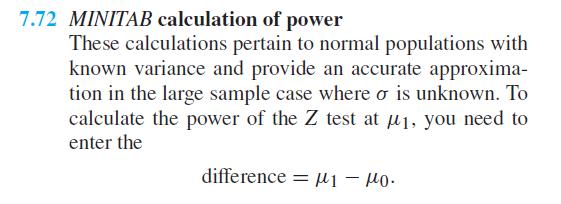
MINITAB calculation of power These calculations pertain to normal populations with known variance and provide an accurate approximation in the large sample case where \(\sigma\) is unknown. To calculate the power of the \(Z\) test at \(\mu_{1}\), you need to enter the\[\text { difference
Use computer software to repeat Exercise 7.71.Data From Exercise 7.71 77 7.71 Refer to the example concerning average sound inten- sity on page 260. Calculate the power at when (a) the level is changed to a = 0.03. = (b) = 0.05 but the alternative is changed to the two- sided H 75.2.
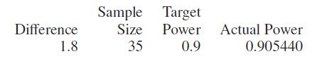
MINITAB calculation of sample size Refer to Exercise 7.72, but this time leave Sample size blank but Type 0.90 in power to obtain the partial output concerning sample sizeRefer to the example concerning sound intensity on page 260 . Find the required sample size if power must be at least 0.96 at
MINITAB calculation of power or OC curve Refer to the steps in Exercise 7.72, but enter a range of values for the difference.Here 0:3/.1 goes in steps from 0 to 3 in steps of . 1 for Example 22.With reference to the electric car battery example on page 242, use computer software to obtain the power
Specify the null hypothesis and the alternative hypothesis in each of the following cases.(a) An engineer hopes to establish that an additive will increase the viscosity of an oil.(b) An electrical engineer hopes to establish that a modified circuit board will give a computer a higher average
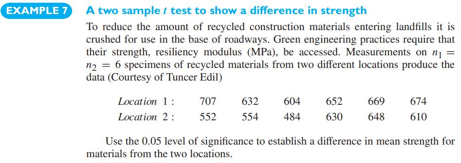
With reference to Example 7 on page 29, find a 95% confidence interval for the mean strength of the aluminum alloy.Data From Example 7 EXAMPLE 7 A two sample t test to show a difference in strength To reduce the amount of recycled construction materials entering landfills it is crushed for use in
While performing a certain task under simulated weightlessness, the pulse rate of 32 astronaut trainees increased on the average by 26.4 beats per minute with a standard deviation of 4.28 beats per minute. What can one assert with \(95 \%\) confidence about the maximum error if \(\bar{x}=26.4\) is
It is desired to estimate the mean number of hours of continuous use until a printer overheats. If it can be assumed that \(\sigma=4\) hours, how large a sample is needed so that one will be able to assert with \(95 \%\) confidence that the sample mean is off by at least 15 hours?
A sample of 15 pneumatic thermostats intended for use in a centralized heating unit has an average output pressure of \(9 \mathrm{psi}\) and a standard deviation of \(1.5 \mathrm{psi}\). Assuming the data may be treated as a random sample from a normal population, determine a \(90 \%\) confidence
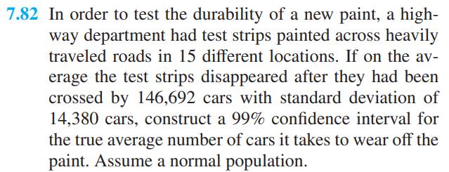
In order to test the durability of a new paint, a highway department had test strips painted across heavily traveled roads in 15 different locations. If on the average the test strips disappeared after they had been crossed by 146,692 cars with standard deviation of 14,380 cars, construct a \(99
Referring to Exercise 7.82 and using 14,380 as an estimate of \(\sigma\), find the sample size that would have been needed to be able to assert with \(95 \%\) confidence that the sample mean is off by at most 10,000. First estimate \(n_{1}\) by using \(z=1.96\), then use \(t_{0.025}\) for
A laboratory technician is timed 20 times in the performance of a task, getting \(\bar{x}=7.9\) and \(s=1.2 \mathrm{~min}-\) utes. If the probability of a Type I error is to be at most 0.05 , does this constitute evidence against the null hypothesis that the average time is less than or equal to
In a fatigue study, the time spent working by employees in a factory was observed. The ten readings (in hours) were\[\begin{array}{llllllllll}4.8 & 3.6 & 10.8 & 5.7 & 8.2 & 6.8 & 7.5 & 7.7 & 6.3 & 8.6\end{array}\]Assuming the population sampled is normal, construct a \(90 \%\) confidence interval
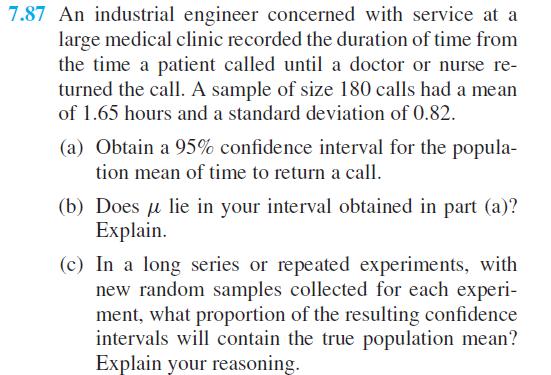
An industrial engineer concerned with service at a large medical clinic recorded the duration of time from the time a patient called until a doctor or nurse returned the call. A sample of size 180 calls had a mean of 1.65 hours and a standard deviation of 0.82 .(a) Obtain a 95\% confidence interval
Refer to Exercise 7.87.(a) Perform a test with the intention of establishing that the mean time to return a call is greater than 1.5 hours. Use \(\alpha=0.05\).(b) In light of your conclusion in part (a), what error could you have made? Explain in the context of this problem.(c) In a long series of
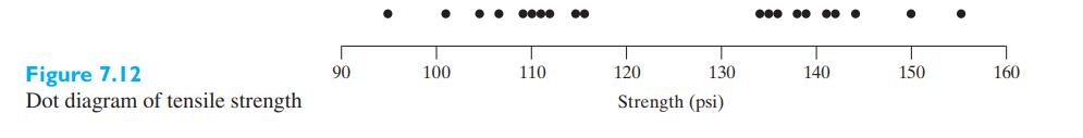
The compressive strength of parts made from a composite material are known to be nearly normally distributed. A scientist, using the testing device for the first time, obtains the tensile strength (psi) of 20 specimens\[\begin{array}{rlllllllll}95 & 102 & 105 & 107 & 109 & 110
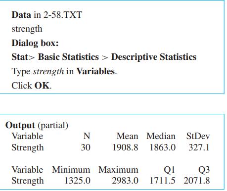
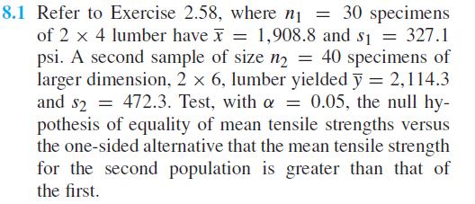
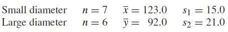
Refer to Exercise 2.58, where \(n_{1}=30\) specimens of \(2 \times 4\) lumber have \(\bar{x}=1,908.8\) and \(s_{1}=327.1\) psi. A second sample of size \(n_{2}=40\) specimens of larger dimension, \(2 \times 6\), lumber yielded \(\bar{y}=2,114.3\) and \(s_{2}=472.3\). Test, with \(\alpha=0.05\), the
Refer to Exercise 8.1 and obtain a \(95 \%\) confidence interval for the difference in mean tensile strength.Data From Exercise 8.1 Data From Exercise 2.58 8.1 Refer to Exercise 2.58, where n = 30 specimens of 2 x 4 lumber have x = 1,908.8 and s = 327.1 psi. A second sample of size n = 40
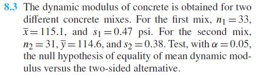
The dynamic modulus of concrete is obtained for two different concrete mixes. For the first mix, \(n_{1}=33\), \(\bar{x}=115.1\), and \(s_{1}=0.47\) psi. For the second mix, \(n_{2}=31, \bar{y}=114.6\), and \(s_{2}=0.38\). Test, with \(\alpha=0.05\), the null hypothesis of equality of mean dynamic
Refer to Exercise 8.3 and obtain a \(95 \%\) confidence interval for the difference in mean dynamic modulus.Data From Exercise 8.3 8.3 The dynamic modulus of concrete is obtained for two different concrete mixes. For the first mix, n = 33, x=115.1, and s = 0.47 psi. For the second mix, n2
An investigation of two types of bulldozers showed that 50 failures of one type of bulldozer took on an average 6.8 hours to repair with a standard deviation of 0.85 hours, while 50 failures of the other type of bulldozer took on an average 7.3 hours to repair with a standard deviation of 1.2
Studying the flow of traffic at two busy intersections between 4 P.M. and 6 P.M. (to determine the possible need for turn signals), it was found that on 40 weekdays there were on the average 247.3 cars approaching the first intersection from the south that made left turns while on 30 weekdays there
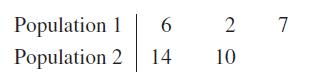
Given the \(n_{1}=3\) and \(n_{2}=2\) observations from Population 1 and Population 2, respectively,(a) Calculate the three deviations \(x-\bar{x}\) and two deviations \(y-\bar{y}\).(b) Use your results from part(a) to obtain the pooled variance. 6 2 7 10 Population 1 Population 2 14
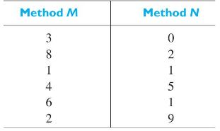
Two methods for manufacturing a product are to be compared. Given 12 units, six are manufactured using method \(M\) and six are manufactured using method \(N\).(a) How would you assign manufacturing methods to the 12 units?(b) The response is the percent of finished product that did not meet
Measuring specimens of nylon yarn taken from two spinning machines, it was found that 8 specimens from the first machine had a mean denier of 9.67 with a standard deviation of 1.81 , while 10 specimens from the second machine had a mean denier of 7.43 with a standard deviation of 1.48. Assuming
We know that silk fibers are very tough but in short supply. Breakthroughs by one research group result in the summary statistics for the stress \((\mathrm{MPa})\) of synthetic silk fibers (Source: F. Teulé, et. al. (2012), Combining flagelliform and dragline spider silk motifs to produce tunable
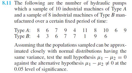
The following are the number of hydraulic pumps which a sample of 10 industrial machines of Type \(A\) and a sample of 8 industrial machines of Type \(B\) manufactured over a certain fixed period of time:\(\begin{array}{lllllllllll}\text { Type A: } & 8 & 6 & 7 & 9 & 4 & 11 & 8 & 10 & 6 &
With reference to Example 5 construct a 95% confidence interval for the true difference between the average resistance of the two kinds of wire.Data From Example 5 EXAMPLE 5 The multiplication rule with k = 12 stages of choices If a test consists of 12 true-false questions, in how many different
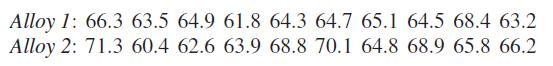
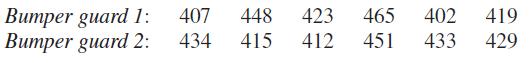
In each of the parts below, first decide whether or not to use the pooled estimator of variance. Assume that the populations are normal.(a) The following are the Brinell hardness values obtained for samples of two magnesium alloys before testing:Use the 0.05 level of significance to test the null
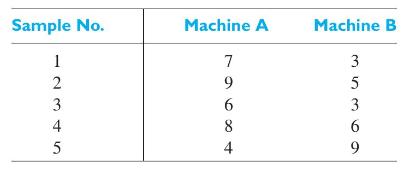
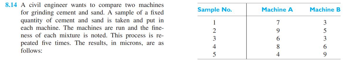
A civil engineer wants to compare two machines for grinding cement and sand. A sample of a fixed quantity of cement and sand is taken and put in each machine. The machines are run and the fineness of each mixture is noted. This process is repeated five times. The results, in microns, are as
Refer to Exercise 8.14. Test with \(\alpha=0.01\), that the mean difference is 0 versus a two-sided alternative.Data From Exercise 8.14Find a 99% confidence interval for the mean difference in machine readings assuming the differences have a normal distribution. 8.14 A civil engineer wants to
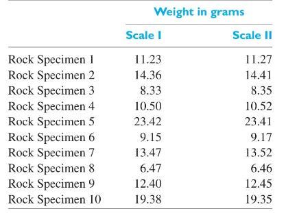
The following data were obtained in an experiment designed to check whether there is a systematic difference in the weights obtained with two different scales:Use the paired \(t\) test at the 0.05 level of significance to try to establish that the mean difference of the weights obtained with the
Refer to Example 14 concerning suspended solids in effluent from a treatment plant. Take the square root of each of the measurements and then take the difference.(a) Construct a \(95 \%\) confidence interval for \(\mu_{D}\).(b) Conduct a level \(\alpha=0.05\) level test of \(H_{0}: \mu_{D}=\) 0
Refer to Example 14 concerning suspended solids in effluent from a treatment plant. Take the natural logarithm of each of the measurements and then take the difference.(a) Construct a 95% confidence interval for \(\mu_{D}\).(b) Conduct a level \(\alpha=0.05\) level test of \(H_{0}: \mu_{D}=\) 0
A shoe manufacturer wants potential customers to compare two types of shoes, one made of the current PVC material \(X\) and one made of a new PVC material \(Y\). Shoes made of both are available. Each person, in a sample of 52, is asked to wear one pair of each type for a whole day. After a walk of
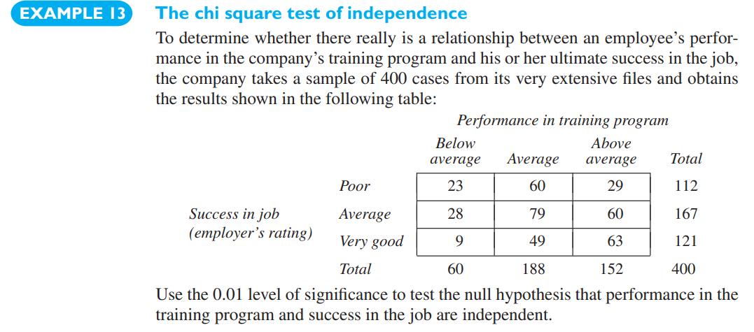
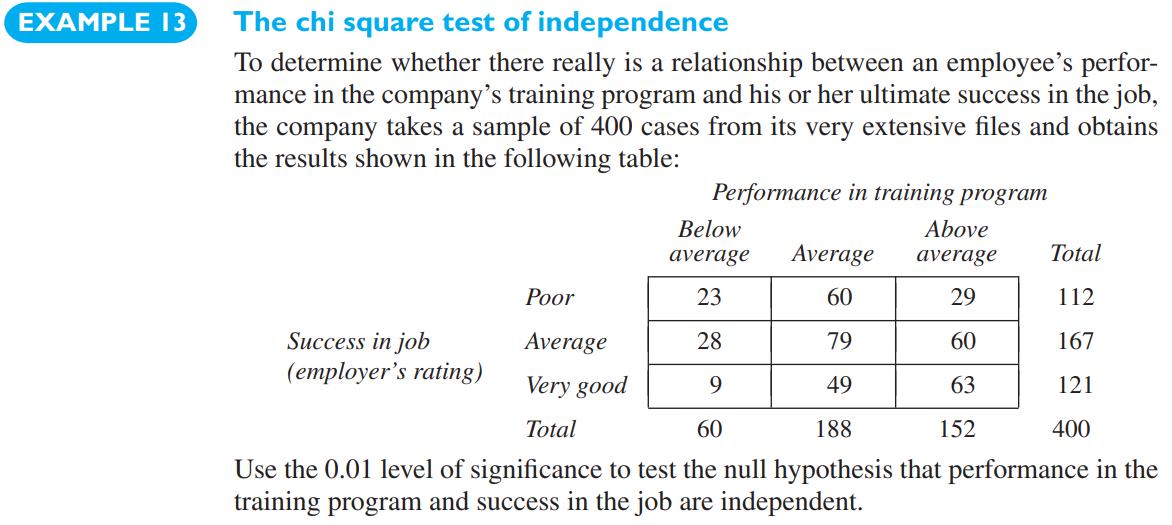
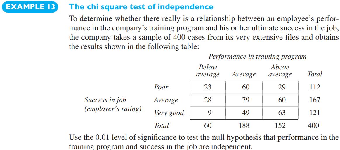
Referring to Example 13, conduct a test to show that the mean change \(\mu_{D}\) is different from 0 . Take \(\alpha=0.05\).Data From Example 13 EXAMPLE 13 The chi square test of independence To determine whether there really is a relationship between an employee's perfor- mance in the company's
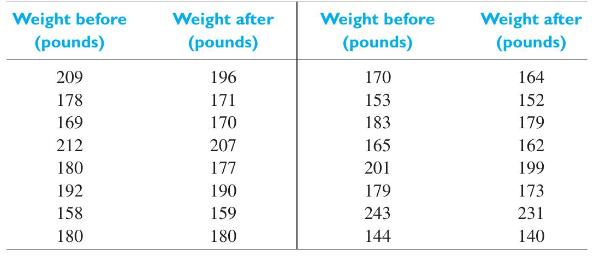
In a study of the effectiveness of physical exercise in weight reduction, a group of 16 persons engaged in a prescribed program of physical exercise for one month showed the following results:Use the 0.01 level of significance to test whether the prescribed program of exercise is effective. Weight
An engineer wants to compare two busy hydraulic belts by recording the number of finished goods that are successfully transferred by the belts in a day. Describe how to select 3 of the next 6 working days to try Belt A. Belt B would then be tried on the other 3 days.
An electrical engineer has developed a modified circuit board for elevators. Suppose 3 modified circuit boards and 6 elevators are available for a comparative test of the old versus the modified circuit boards.(a) Describe how you would select the 3 elevators in which to install the modified
It takes an average of 30 classes for an instructor to teach a civil engineering student probability. The instructor introduces a new software which they feel will lead to faster calculations. The instructor intends to teach 10 students with the new software and compare their calculation times with
How would you randomize, for a two sample test, if 50 cars are available for an emissions study and you want to compare a modified air pollution device with that used in current production?
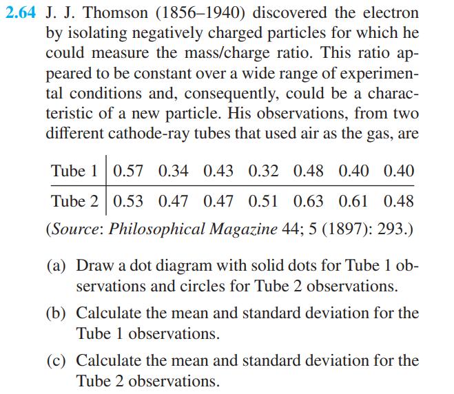
With reference to Exercise 2.64, test that the mean charge of the electron is the same for both tubes. Use \(\alpha=0.05\).Data From Exercise 2.64 2.64 J. J. Thomson (1856-1940) discovered the electron by isolating negatively charged particles for which he could measure the mass/charge ratio. This
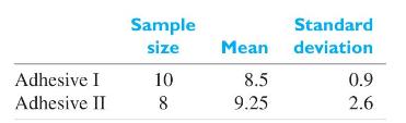
Two adhesives for pasting plywood boards are to be compared. 10 tubes are prepared using Adhesive I and 8 tubes are prepared using Adhesive II. Then 18 different pairs of plywood boards are pasted together, one tube per pair of boards.(a) The response is the time in minutes for the boards to stick
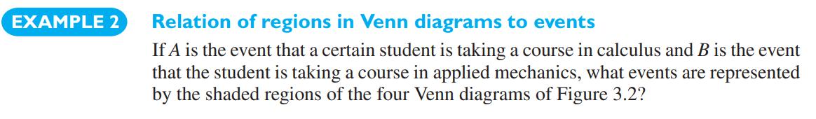
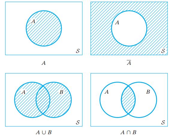
With reference to Example 2, Chapter 2, test that the mean copper content is the same for both heats.Data From Example 2Data From Figure 3.2 EXAMPLE 2 Relation of regions in Venn diagrams to events If A is the event that a certain student is taking a course in calculus and B is the event that the
Random samples are taken from two normal populations with \(\sigma_{1}=9.6\) and \(\sigma_{2}=13.2\) to test the null hypothesis \(\mu_{1}-\mu_{2}=41.2\) against the alternative hypothesis \(\mu_{1}-\mu_{2}>41.2\) at the level of significance \(\alpha=0.05\). Determine the common sample size
With reference to Example 8, find a \(90 \%\) confidence interval for the difference of mean strengths of the alloys(a) using the pooled procedure;(b) using the large samples procedure.Data From Example 8 EXAMPLE 8 Evaluating a combination In how many different ways can 3 of 18 automotive engineers
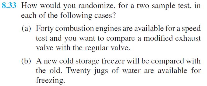
How would you randomize, for a two sample test, in each of the following cases?(a) Forty combustion engines are available for a speed test and you want to compare a modified exhaust valve with the regular valve.(b) A new cold storage freezer will be compared with the old. Twenty jugs of water are
With reference to part(a) of Exercise 8.33, how would you pair and then randomize for a paired test?Data From Exercise 8.33 8.33 How would you randomize, for a two sample test, in each of the following cases? (a) Forty combustion engines are available for a speed test and you want to compare a
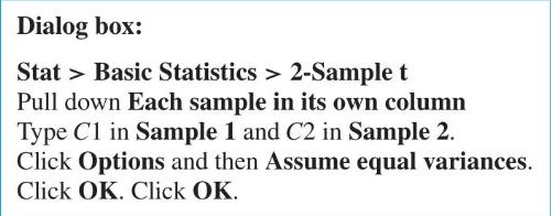
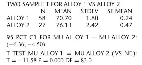
Two samples in \(\mathrm{C} 1\) and \(\mathrm{C} 2\) can be analyzed using the MINITAB commandsIf you do not click Assume equal variances, the Smith-Satterthwaite test is performed.The output relating to Example 8 isPerform the test for the data in Exercise 8.11.Data From Exercise 8.11Data From
Refer to Example 13 concerning an array of sites that smell toxic chemicals. When exposed to the common manufacturing chemical Arsine, a product of arsenic and acid, the change in the red component is measured six times. (Courtesy of the authors)\[\begin{array}{llllll}0.10 & -0.33 & -1.12
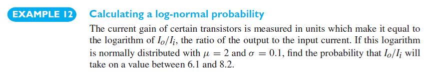
Refer to Example 12 concerning the improvement in lost worker-hours. Obtain a \(90 \%\) confidence interval for the mean of this paired difference.Data From Example 12 EXAMPLE 12 Calculating a log-normal probability The current gain of certain transistors is measured in units which make it equal to
Showing 6100 - 6200
of 7136
First
55
56
57
58
59
60
61
62
63
64
65
66
67
68
69
Last
Step by Step Answers