New Semester
Started
Get
50% OFF
Study Help!
--h --m --s
Claim Now
Question Answers
Textbooks
Find textbooks, questions and answers
Oops, something went wrong!
Change your search query and then try again
S
Books
FREE
Study Help
Expert Questions
Accounting
General Management
Mathematics
Finance
Organizational Behaviour
Law
Physics
Operating System
Management Leadership
Sociology
Programming
Marketing
Database
Computer Network
Economics
Textbooks Solutions
Accounting
Managerial Accounting
Management Leadership
Cost Accounting
Statistics
Business Law
Corporate Finance
Finance
Economics
Auditing
Tutors
Online Tutors
Find a Tutor
Hire a Tutor
Become a Tutor
AI Tutor
AI Study Planner
NEW
Sell Books
Search
Search
Sign In
Register
study help
business
introduction to probability statistics
Probability And Statistics For Engineers 9th Global Edition Richard Johnson, Irwin Miller, John Freund - Solutions
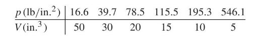
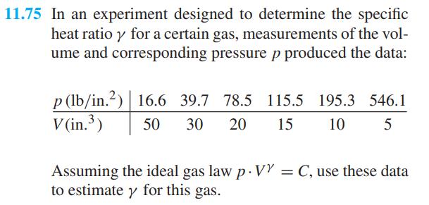
In an experiment designed to determine the specific heat ratio \(\gamma\) for a certain gas, measurements of the volume and corresponding pressure \(p\) produced the data:Assuming the ideal gas law \(p \cdot V^{\gamma}=C\), use these data to estimate \(\gamma\) for this gas. p(lb/in.) 16.6 39.7
With reference to Exercise 11.75, use the method of Section 11.2 to construct a \(95 \%\) confidence interval for \(\gamma\). State what assumptions will have to be made.Data From Exercise 11.75 11.75 In an experiment designed to determine the specific heat ratio y for a certain gas, measurements
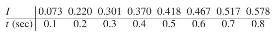
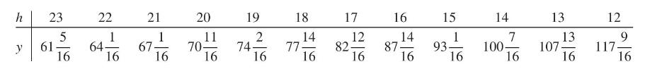
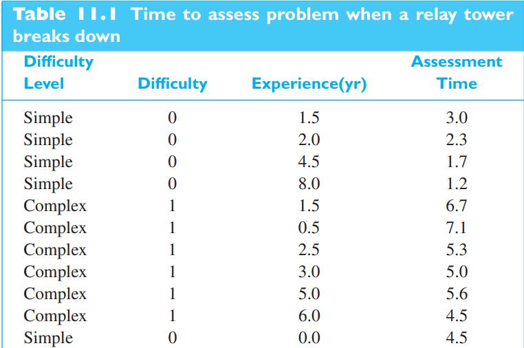
The rise of current in an inductive circuit having the time constant \(\tau\) is given by\[I=1-e^{-t / \tau}\]where \(t\) is the time measured from the instant the switch is closed, and \(I\) is the ratio of the current at time \(t\) to the full value of the current given by Ohm's law. Given the
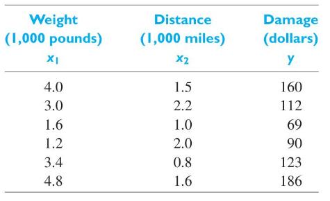
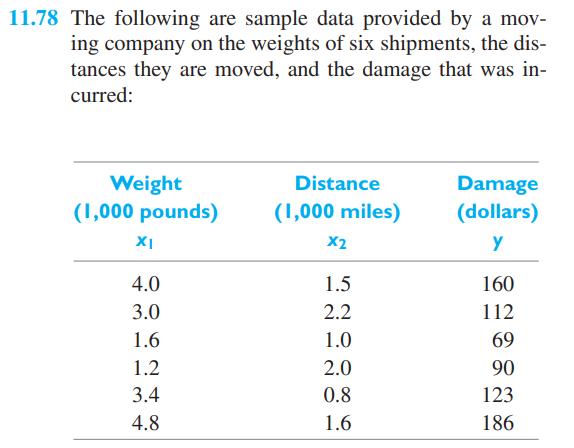
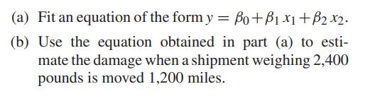
The following are sample data provided by a moving company on the weights of six shipments, the distances they are moved, and the damage that was incurred:(a) Fit an equation of the form \(y=\beta_{0}+\beta_{1} x_{1}+\beta_{2} x_{2}\).(b) Use the equation obtained in part (a) to estimate the damage
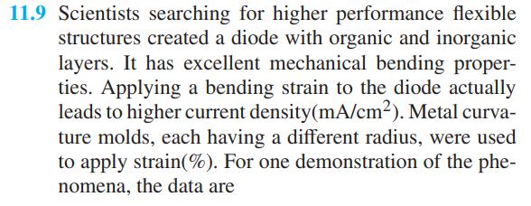
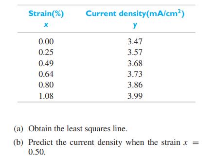
With reference to Exercise 11.9,(a) find a 95% confidence interval for the mean current density when the strain is \(x=0.50\);(b) find 95% limits of prediction for the current density when a new diode has stress \(x=0.50\).Data From Exercise 11.9 11.9 Scientists searching for higher performance
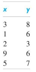
Use the expression on page 367, involving deviations from the mean, to calculate \(r\) for the following data: x Y 3 8 6 367 -205
If \(r=0.41\) for one set of paired data and \(r=0.29\) for another, compare the strengths of the two relationships.
If for certain paired data \(n=18\) and \(r=0.44\), test the null hypothesis \(ho=0.30\) against the alternative hypothesis \(ho>0.30\) at the 0.01 level of significance.
Assuming that the necessary assumptions are met, construct a 95\% confidence interval for \(ho\) when(a) \(r=0.78\) and \(n=15\);(b) \(r=-0.62\) and \(n=32\);(c) \(r=0.17\) and \(n=35\).
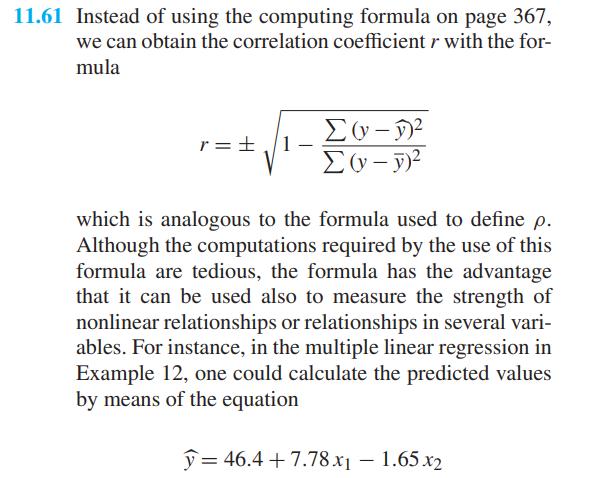
With reference to Exercise 11.78, use the theory of Exercise 11.61 to calculate the multiple correlation coefficient (which measures how strongly the damage is related to both weight and distance).Data From Exercise 11.78Data From Exercise 11.61 11.78 The following are sample data provided by a
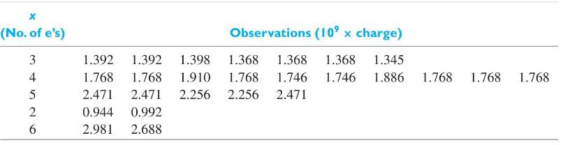
Robert A. Millikan (1865-1953) produced the first accurate measurements on the charge \(e\) of an electron. He devised a method to observe a single drop of water or oil under the influence of both electric and gravitational fields. Usually, a droplet carried multiple electrons, and direct
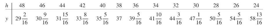
Robert Boyle (1627-1691) established the law that (pressure \(\times\) volume) \(=\) constant for a gas at a constant temperature. By pouring mercury into the open top of the long side of a \(\mathrm{J}\)-shaped tube, he increased the pressure on the air trapped in the short leg. The volume of
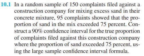
In a random sample of 150 complaints filed against a construction company for mixing excess sand in their concrete mixture, 95 complaints showed that the proportion of sand in the mix exceeded 75 percent. Construct a \(90 \%\) confidence interval for the true proportion of complaints filed against
With reference to Exercise 10.1, what can we say with \(95 \%\) confidence about the maximum error if we use the sample proportion as an estimate of the true proportion of complaints filed against this construction company where the proportion of sand exceeds 75 percent?Data From Exercise 10.1 10.1
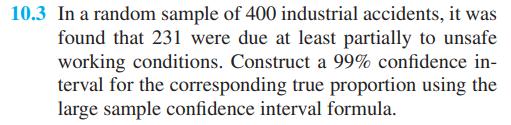
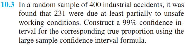
In a random sample of 400 industrial accidents, it was found that 231 were due at least partially to unsafe working conditions. Construct a \(99 \%\) confidence interval for the corresponding true proportion using the large sample confidence interval formula.
With reference to Exercise 10.3, what can we say with \(95 \%\) confidence about the maximum error if we use the sample proportion to estimate the corresponding true proportion?Data From Exercise 10.3 10.3 In a random sample of 400 industrial accidents, it was found that 231 were due at least
In a random sample of 140 observations of workers on a site, 25 were found to be idle. Construct a \(99 \%\) confidence interval for the true proportion of workers found idle, using the large sample confidence interval formula.
In an experiment, 85 of 125 processors were observed to process data at a speed of 4,700 MIPS. If we estimate the corresponding true proportion as \(\frac{85}{125}=0.68\), what can we say with \(99 \%\) confidence about the maximum error?
Among 100 fish caught in a large lake, 18 were inedible due to the pollution of the environment. If we use \(\frac{18}{100}=0.18\) as an estimate of the corresponding true proportion, with what confidence can we assert that the error of this estimate is at most 0.065 ?
New findings suggest many persons possess symptoms of motion sickness after watching a 3D movie. One scientist administered a questionnaire to \(n=451\) adults after they watched a 3D movie of their choice. Based on these self-reported results, 247 are determined to have some motion sickness.
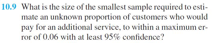
What is the size of the smallest sample required to estimate an unknown proportion of customers who would pay for an additional service, to within a maximum error of 0.06 with at least \(95 \%\) confidence?
With reference to Exercise 10.9, how would the required sample size be affected if it is known that the proportion to be estimated is at least 0.75 ?Data From Exercise 10.9 10.9 What is the size of the smallest sample required to esti- mate an unknown proportion of customers who would pay for an
Suppose that we want to estimate what percentage of all bearings wears out due to friction within a year of installation. How large a sample will we need to be at least \(90 \%\) confident that the error of our estimate, the sample percentage, is at most \(2.25 \%\) ?
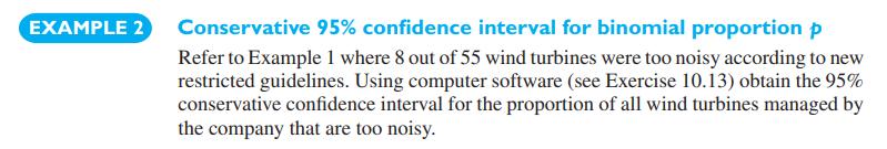
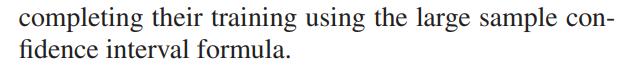
Refer to Example 1. How large a sample of wind turbines is needed to ensure that, with at least \(95 \%\) confidence, the error in our estimate of the sample proportion is at most 0.06 if(a) nothing is known about the population proportion?(b) the population proportion is known not to exceed 0.20
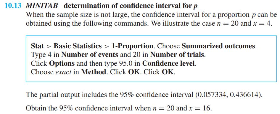
MINITAB determination of confidence interval for \(p\)When the sample size is not large, the confidence interval for a proportion \(p\) can be obtained using the following commands. We illustrate the case \(n=20\) and \(x=4\).The partial output includes the \(95 \%\) confidence interval
Use Exercise 10.13 or other software to obtain the interval requested in Exercise 10.3.Data From Exercise 10.13 10.13 MINITAB determination of confidence interval for p When the sample size is not large, the confidence interval for a proportion p can be obtained using the following commands. We
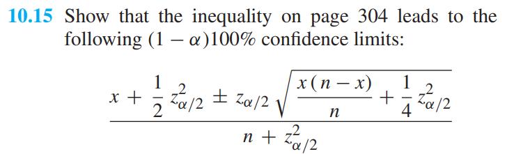
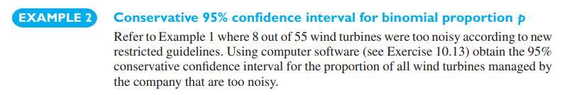
Show that the inequality on page 304 leads to the following \((1-\alpha) 100 \%\) confidence limits:\[\frac{x+\frac{1}{2} z_{\alpha / 2}^{2} \pm z_{\alpha / 2} \sqrt{\frac{x(n-x)}{n}+\frac{1}{4} z_{\alpha / 2}^{2}}}{n+z_{\alpha / 2}^{2}}\] EXAMPLE 2 Conservative 95% confidence interval for binomial
Use the formula of Exercise 10.15 to rework Exercise 10.3.Data From Exercise 10.3Data From Exercise 10.15 10.3 In a random sample of 400 industrial accidents, it was found that 231 were due at least partially to unsafe working conditions. Construct a 99% confidence in- terval for the corresponding
A chemical laboratory was facing issues with the concentration of the sulfuric acid they prepared. The first step was to collect data on the magnitude of the problem. Of 5,186 recently supplied acid vials, 846 had concentration issues that could easily be detected by a basic chemical test. Obtain a
An international corporation needed several millions of words, from thousands of documents and manuals, translated. The work was contracted to a company that used computer-assisted translation, along with some human checks. The corporation conducted its own quality check by sampling the
A manufacturer of submersible pumps claims that at most \(30 \%\) of the pumps require repairs within the first 5 years of operation. If a random sample of 120 of these pumps includes 47 which required repairs within the first 5 years, test the null hypothesis \(p=0.30\) against the alternative
A supplier of imported vernier calipers claims that \(90 \%\) of their instruments have a precision of 0.999. Testing the null hypothesis \(p=0.90\) against the alternative hypothesis \(p eq 0.90\), what can we conclude at the level of significance \(\alpha=0.10\), if there were 665 calipers out of
To check on an ambulance service's claim that at least \(40 \%\) of its calls are life-threatening emergencies, a random sample was taken from its files, and it was found that only 49 of 150 calls were life-threatening emergencies. Can the null hypothesis \(p=0.40\) be rejected against the
In a random sample of 600 cars making a right turn at a certain intersection, 157 pulled into the wrong lane. Test the null hypothesis that actually \(30 \%\) of all drivers make this mistake at the given intersection, using the alternative hypothesis \(p eq 0.30\) and the level of significance(a)
An airline claims that only \(6 \%\) of all lost luggage is never found. If, in a random sample, 17 of 200 pieces of lost luggage are not found, test the null hypothesis \(p=0.06\) against the alternative hypothesis \(p>0.06\) at the 0.05 level of significance.
Suppose that 4 of 13 undergraduate engineering students are going on to graduate school. Test the dean's claim that \(60 \%\) of the undergraduate students will go on to graduate school, using the alternative hypothesis \(p
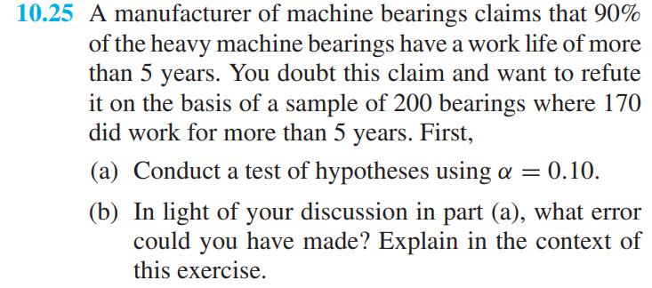
A manufacturer of machine bearings claims that \(90 \%\) of the heavy machine bearings have a work life of more than 5 years. You doubt this claim and want to refute it on the basis of a sample of 200 bearings where 170 did work for more than 5 years. First,(a) Conduct a test of hypotheses using
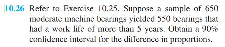
Refer to Exercise 10.25. Suppose a sample of 650 moderate machine bearings yielded 550 bearings that had a work life of more than 5 years. Obtain a \(90 \%\) confidence interval for the difference in proportions.Data From Exercise 10.25 10.26 Refer to Exercise 10.25. Suppose a sample of 650
Tests are made on the proportion of defective castings produced by 5 different molds. If there were 14 defectives among 100 castings made with Mold I, 33 defectives among 200 castings made with Mold II, 21 defectives among 180 castings made with Mold III, 17 defectives among 120 castings made with
A study showed that 64 of 180 persons who saw a photocopying machine advertised during the telecast of a baseball game and 75 of 180 other persons who saw it advertised on a variety show remembered the brand name 2 hours later. Use the \(\chi^{2}\) statistic to test at the 0.05 level of
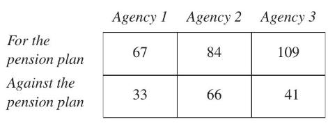
The following data come from a study in which random samples of the employees of three government agencies were asked questions about their pension plan:Use the 0.01 level of significance to test the null hypothesis that the actual proportions of employees favoring the pension plan are the same.
A factory owner must decide which of two alternative electric generator systems should be installed in their factory. If each generator is tested 175 times and the first generator fails to work (does not start or does not transmit electricity) 15 times and the second generator fails to work 25
With reference to the preceding exercise, verify that the square of the value obtained for \(Z\) in part (b) equals the value obtained for \(\chi^{2}\) in part (a).
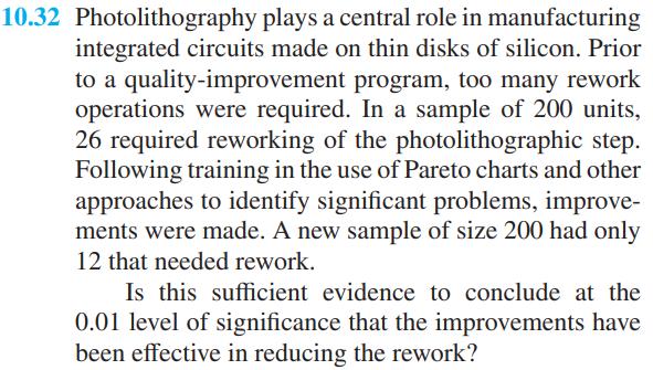
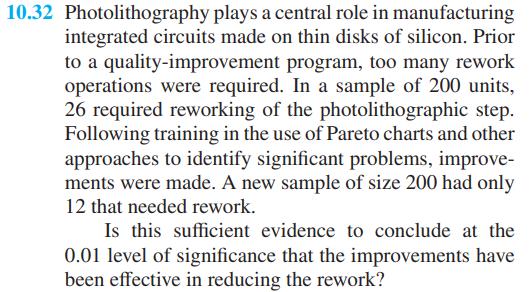
Photolithography plays a central role in manufacturing integrated circuits made on thin disks of silicon. Prior to a quality-improvement program, too many rework operations were required. In a sample of 200 units, 26 required reworking of the photolithographic step. Following training in the use of
With reference to Exercise 10.32, find a large sample 99% confidence interval for the true difference of the proportions.Data From Exercise 10.32 10.32 Photolithography plays a central role in manufacturing integrated circuits made on thin disks of silicon. Prior to a quality-improvement program,
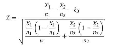
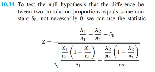
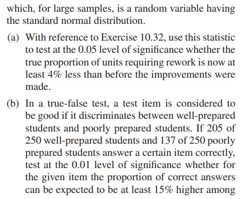
To test the null hypothesis that the difference between two population proportions equals some constant \(\delta_{0}\), not necessarily 0 , we can use the statisticwhich, for large samples, is a random variable having the standard normal distribution.(a) With reference to Exercise 10.32, use this
With reference to part (b) of Exercise 10.34, find a large sample \(99 \%\) confidence interval for the true difference of the proportions.Data From Exercise 10.34 10.34 To test the null hypothesis that the difference be- tween two population proportions equals some con- stant 80, not necessarily
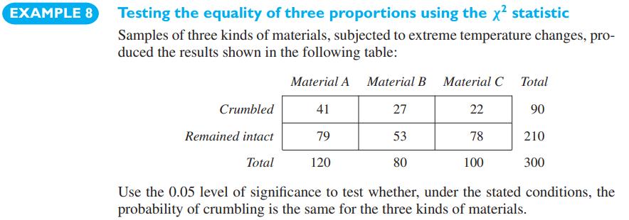
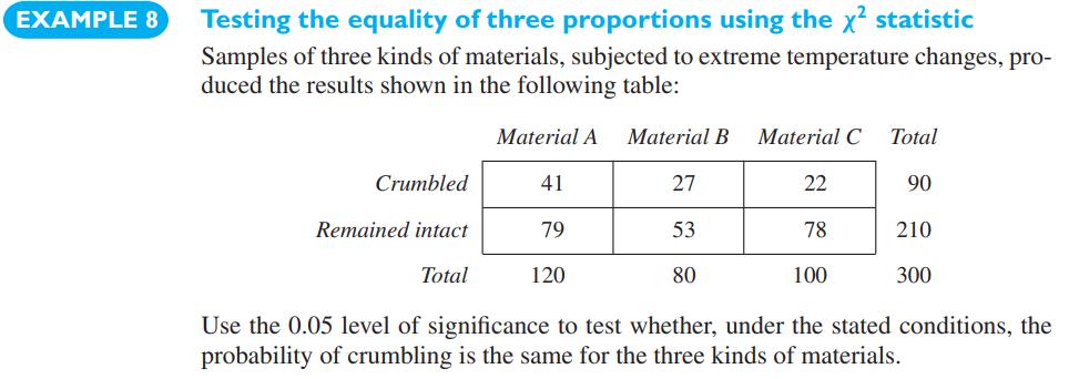
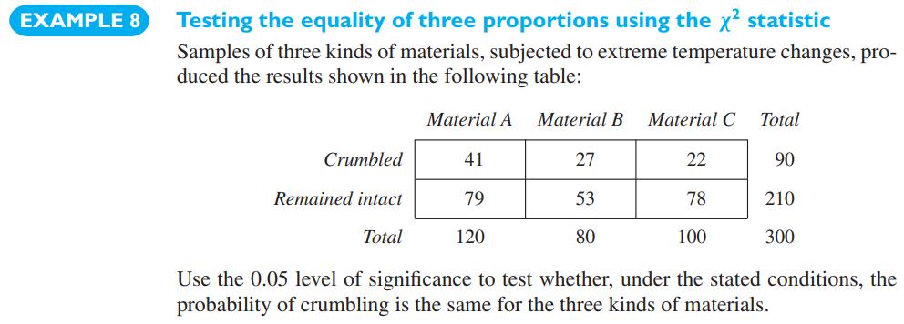
Verify that the formulas for the \(\chi^{2}\) statistic on page 311 (with \(\widehat{p}\) substituted for the \(p_{i}\) ) and on page 312 are equivalent. EXAMPLE 8 Testing the equality of three proportions using the x statistic Samples of three kinds of materials, subjected to extreme temperature
Verify that if the expected frequencies are determined in accordance with the rule on page 312 , the sum of the expected frequencies for each row and column equals the sum of the corresponding observed frequencies.
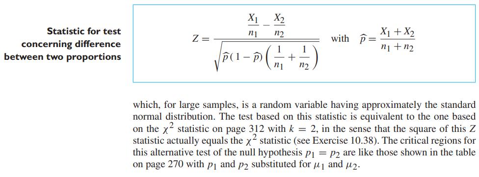
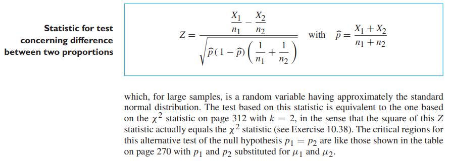
Verify that the square of the \(Z\) statistic on page 314 equals the \(\chi^{2}\) statistic on page 312 for \(k=2\). Statistic for test concerning difference between two proportions X1 X2 n1 - n2 Z = P(1 P(1 - p) + 12 with p= X + X2 = n1+n2 which, for large samples, is a random variable having
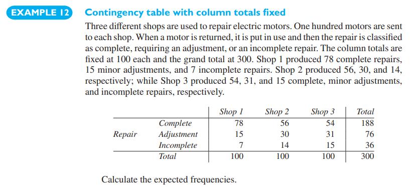
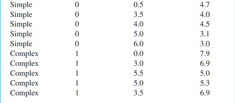
Referring to Example 12 and the data on repair, use the 0.05 level of significance to test whether there is homogeneity among the shops' repair distributions.Data From Example 12 EXAMPLE 12 Contingency table with column totals fixed Three different shops are used to repair electric motors. One
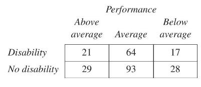
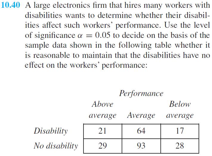
A large electronics firm that hires many workers with disabilities wants to determine whether their disabilities affect such workers' performance. Use the level of significance \(\alpha=0.05\) to decide on the basis of the sample data shown in the following table whether it is reasonable to
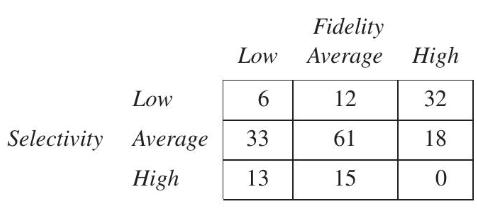
Tests of the fidelity and the selectivity of 190 digital radio receivers produced the results shown in the following table:Use the 0.01 level of significance to test whether there is a relationship (dependence) between fidelity and selectivity. Fidelity Low Average Average High Low 6 12 32
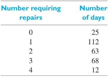
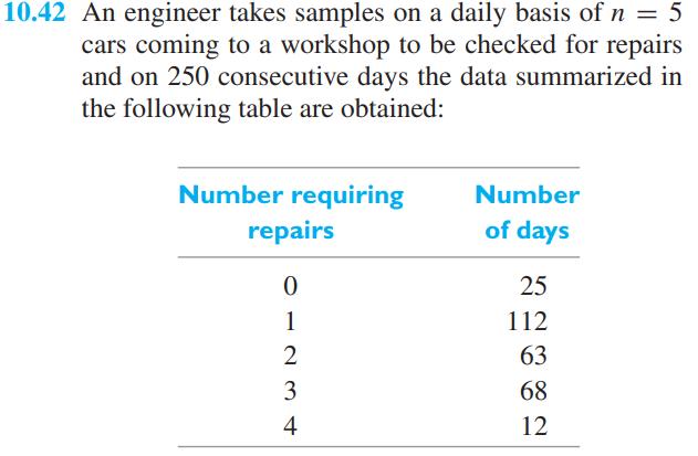
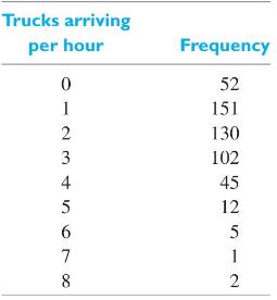
An engineer takes samples on a daily basis of \(n=5\) cars coming to a workshop to be checked for repairs and on 250 consecutive days the data summarized in the following table are obtained:To test the claim that \(20 \%\) of all cars coming to the workshop need to be repaired, look up the
With reference to Exercise 10.42, verify that the mean of the observed distribution is 1.6 , corresponding to \(40 \%\) of the cars requiring repairs. Then look up the probabilities for \(n=5\) and \(p=0.25\) in Table 1, calculate the expected frequencies, and test at the 0.05 level of significance
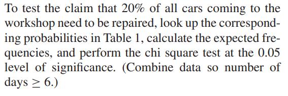
The following is the distribution of the hourly number of trucks arriving at a company's warehouse:Find the mean of this distribution, and using it (rounded to one decimal place) as the parameter \(\lambda\), fit a Poisson distribution. Test for goodness of fit at the 0.05 level of significance.
Among 100 purification filters used in an experiment, 46 had a service life of less than 20 hours, 19 had a service life of 20 or more but less than 40 hours, 17 had a service life of 40 or more but less than 60 hours, 12 had a service life of 60 or more but less than 80 hours, and 6 had a service
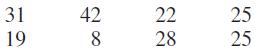
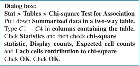
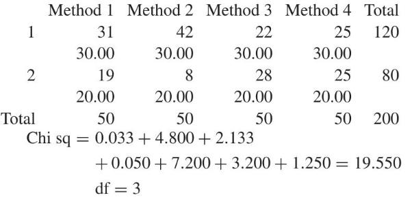
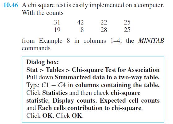
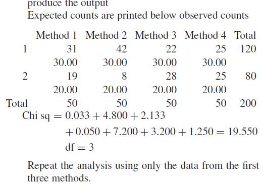
A chi square test is easily implemented on a computer. With the countsfrom Example 8 in columns 1-4, the MINITAB commandsproduce the output Expected counts are printed below observed countsRepeat the analysis using only the data from the first three methods. 31 19 18 42 2223 25 28 25
The procedure in Exercise 10.46 also calculates the chi square test for independence. Do Exercise 10.40 using the computer.Data From Exercise 10.46Data From Exercise 10.40 10.46 A chi square test is easily implemented on a computer. With the counts 31 42 22 25 19 8 28 25 from Example 8 in columns
In a sample of 100 ceramic pistons made for an experimental diesel engine, 18 were cracked. Construct a \(95 \%\) confidence interval for the true proportion of cracked pistons using the large sample confidence interval formula.
With reference to Exercise 10.48, test the null hypothesis \(p=0.20\) versus the alternative hypothesis \(pData From Exercise 10.48 10.48 In a sample of 100 ceramic pistons made for an ex- perimental diesel engine, 18 were cracked. Construct a 95% confidence interval for the true proportion of
In a random sample of 160 workers exposed to a certain amount of radiation, 24 experienced some ill effects. Construct a \(99 \%\) confidence interval for the corresponding true percentage using the large sample confidence interval formula.
With reference to Exercise 10.50, test the null hypothesis \(p=0.18\) versus the alternative hypothesis \(p eq 0.18\) at the 0.01 level.Data From Exercise 10.50 10.50 In a random sample of 160 workers exposed to a certain amount of radiation, 24 experienced some ill effects. Construct a 99%
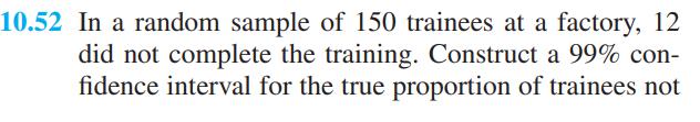
In a random sample of 150 trainees at a factory, 12 did not complete the training. Construct a 99% confidence interval for the true proportion of trainees not completing their training using the large sample confidence interval formula.
With reference to Exercise 10.52, test the hypothesis \(p=0.05\) versus the alternative hypothesis \(p>0.05\) at the 0.05 level.Data From Exercise 10.52 10.52 In a random sample of 150 trainees at a factory, 12 did not complete the training. Construct a 99% con- fidence interval for the true
Refer to Example 5 but suppose there are two additional design plans \(\mathrm{B}\) and \(\mathrm{C}\) for making miniature drones. Under B, 10 of 40 drones failed the initial test and under C 15 of 39 failed. Consider the results for all three design plans. Use the 0.05 level of significance to
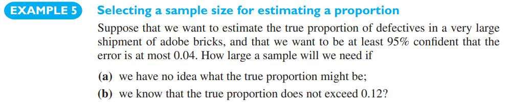
As a check on the quality of eye glasses purchased over the internet, glasses were individually ordered from several different online vendors. Among the 92 lenses with antireflection coating, 61 prescriptions required a thickness at the center greater than \(1.9 \mathrm{~mm}\) and 31 were thinner.
With reference to Exercise 10.55, find a large sample 95% confidence interval for the true difference of probabilities.Data From Exercise 10.55 10.55 As a check on the quality of eye glasses purchased over the internet, glasses were individually ordered from several different online vendors. Among
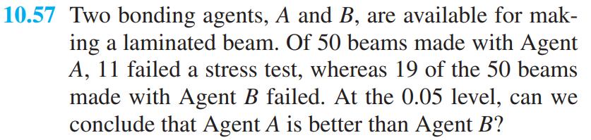
Two bonding agents, \(A\) and \(B\), are available for making a laminated beam. Of 50 beams made with Agent \(A, 11\) failed a stress test, whereas 19 of the 50 beams made with Agent \(B\) failed. At the 0.05 level, can we conclude that Agent \(A\) is better than Agent \(B\) ?
With reference to Exercise 10.57, find a large sample 95% confidence interval for the true difference of the probabilities of failure.Data From Exercise 10.57 10.57 Two bonding agents, A and B, are available for mak- ing a laminated beam. Of 50 beams made with Agent A, 11 failed a stress test,
Cooling pipes at three nuclear power plants are investigated for deposits that would inhibit the flow of water. From 30 randomly selected spots at each plant, 13 from the first plant, 8 from the second plant, and 19 from the third were clogged.(a) Use the 0.05 level to test the null hypothesis of
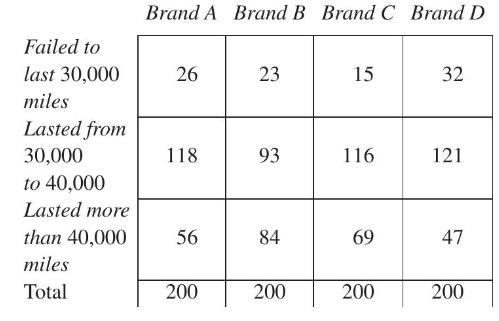
Two hundred tires of each of four brands are individually placed in a testing apparatus and run until failure. The results are obtained the results shown in the following table:(a) Use the 0.01 level of significance to test the null hypothesis that there is no difference in the qual-ity of the four
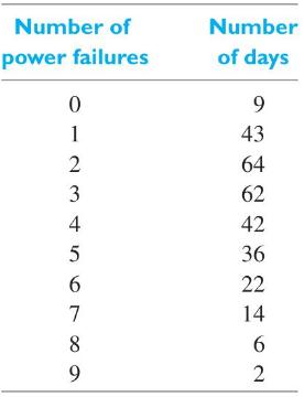
The following is the distribution of the daily number of power failures reported in a western city on 300 days:Test at the 0.05 level of significance whether the daily number of power failures in this city is a random variable having the Poisson distribution with \(\lambda=3.2\). Number of power
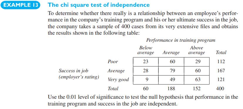
With reference to Example 13, repeat the analysis after combining the categories below average and average in the training program and the categories poor and average in success. Comment on the form of the dependence.Data From Example 13 EXAMPLE 13 The chi square test of independence To determine
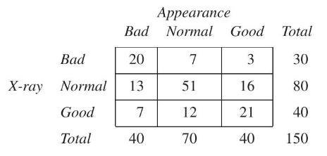
Mechanical engineers, testing a new arc-welding technique, classified welds both with respect to appearance and an X-ray inspection.Test for independence using \(\alpha=0.05\) and find the individual cell contributions to the \(\chi^{2}\) statistic. Appearance Bad Normal Good Total Bad 20 7 3 30
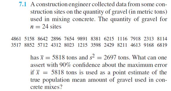
With reference to the previous exercise, construct a 90% confidence interval for the true population mean quantity of gravel in concrete mixes.Data From Previous Exercise 7.1 A construction engineer collected data from some con- struction sites on the quantity of gravel (in metric tons) used in
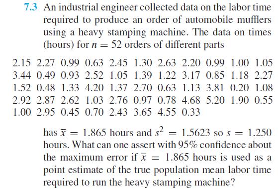
With reference to the previous exercise, construct a 95% confidence interval for the true population mean labor time.Data From Previous Exercise 7.3 An industrial engineer collected data on the labor time required to produce an order of automobile mufflers using a heavy stamping machine. The data
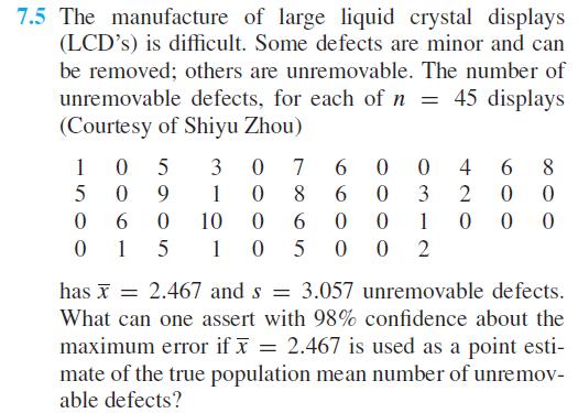
With reference to the previous exercise, construct a 98% confidence interval for the true population mean number of unremovable defects per display.Data From Previous Exercise 7.5 The manufacture of large liquid crystal displays (LCD's) is difficult. Some defects are minor and can be removed;
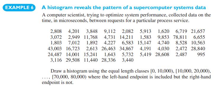
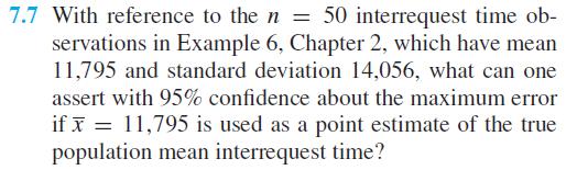
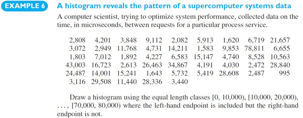
With reference to the \(n=50\) interrequest time observations in Example 6, Chapter 2, which have mean 11,795 and standard deviation 14,056, what can one assert with \(95 \%\) confidence about the maximum error if \(\bar{x}=11,795\) is used as a point estimate of the true population mean
With reference to the previous exercise, construct a 95% confidence interval for the true mean inter-request time.Data From Previous Exercise 7.7 With reference to the n = 50 interrequest time ob- servations in Example 6, Chapter 2, which have mean 11,795 and standard deviation 14,056, what can one
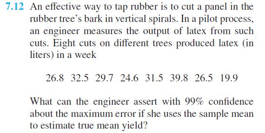
With reference to the previous exercise, assume that production has a normal distribution and obtain a \(99 \%\) confidence interval for the true mean production of the pilot process.Data From Previous Exercise 7.12 An effective way to tap rubber is to cut a panel in the rubber tree's bark in
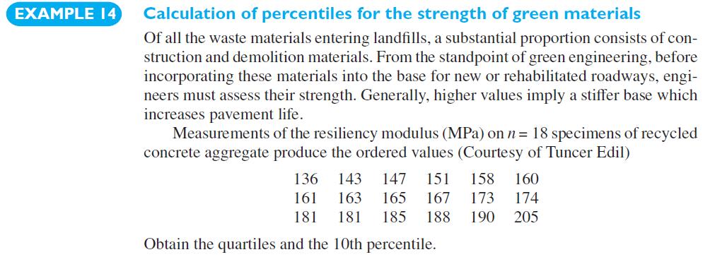
Refer to Example 1 and the data on the resiliency modulus of recycled concrete.(a) Obtain a 95% confidence interval for the population mean resiliency modulus \(\mu\).(b) Is the population mean contained in your interval in part (a)? Explain.(c) What did you assume about the population in your
Suppose that in the preceding exercise the first measurement is recorded incorrectly as 16.0 instead of 14.5. Show that, even though the mean of the sample increases to \(\bar{x}=14.7\), the null hypothesis \(H_{0}: \mu=\) 14.0 is not rejected at level \(\alpha=0.05\). Explain the apparent paradox
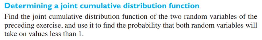
With reference to the preceding exercise, construct a \(95 \%\) confidence interval for the true average increase in the pulse rate of astronaut trainees performing the given task.Data From Preceding Exercise Determining a joint cumulative distribution function Find the joint cumulative
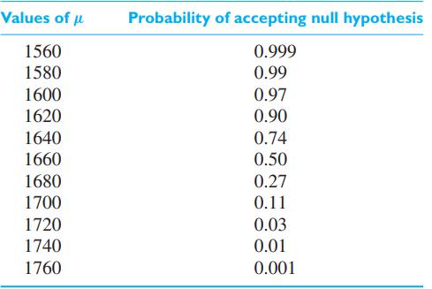
Suppose that in the lithium car battery example on page \(242, n\) is changed from 36 to 50 while the other quantities remain \(\mu_{0}=1600, \sigma=192\), and \(\alpha=\) 0.03. Find(a) the new dividing line of the test criterion;(b) the probability of Type II errors for the values of μ = 1620,
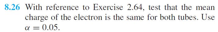
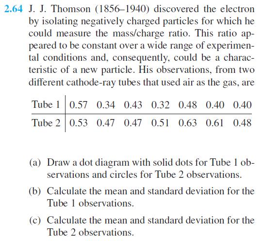
With reference to the previous exercise, find a \(90 \%\) confidence interval for the difference of the two means.Data From Previous Exercise 8.26 With reference to Exercise 2.64, test that the mean charge of the electron is the same for both tubes. Use = 0.05.
With reference to the preceding exercise, find the corresponding distribution function and use it to determine the probabilities that a random variable having this distribution function will take on a value(a) between 0.45 and 0.75 ;(b) less than 0.6.Data From Preceding Exercise Determining a joint
With reference to the preceding exercise, find the corresponding distribution function, and use it to determine the probabilities that a random variable having the distribution function will take on a value(a) greater than 1.8 ;(b) between 0.4 and 1.6 .Data From Preceding Exercise Determining a
With reference to the preceding exercise, for which temperature is the probability 0.05 that it will be exceeded during one day?Data From Preceding Exercise Determining a joint cumulative distribution function Find the joint cumulative distribution function of the two random variables of the
With reference to the preceding exercise, find the probabilities that the random variable will take on a value(a) less than 8.0;(b) between 4.5 and 6.5 .Data From Preceding Exercise Determining a joint cumulative distribution function Find the joint cumulative distribution function of the two
With reference to the preceding exercise, find the marginal densities of the two random variables.Data From Preceding Exercise Determining a joint cumulative distribution function Find the joint cumulative distribution function of the two random variables of the preceding exercise, and use it to
With reference to the preceding exercise, find the joint cumulative distribution function of the two random variables and use it to verify the value obtained for the probability.Data From Preceding Exercise Determining a joint cumulative distribution function Find the joint cumulative distribution
With reference to the preceding exercise, check whether(a) the three random variables are independent;(b) any two of the three random variables are pairwise independent.Data From preceding Exercise Determining a joint cumulative distribution function Find the joint cumulative distribution
A pair of random variables has the circular normal distribution if their joint density is given by\[\begin{aligned}& f\left(x_{1}, x_{2}\right) \\& \quad=\frac{1}{2 \pi \sigma^{2}} e^{-\left[\left(x_{1}-\mu_{1}\right)^{2}+\left(x_{2}-\mu_{2}\right)^{2}\right] / 2 \sigma^{2}} \\& \text {
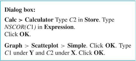
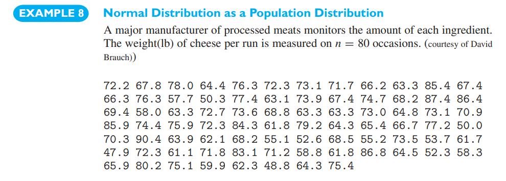
The MINITAB commandswill create a normal scores plot from observations that were set in C1. (MINITAB uses a variant of the normal scores, \(m_{i}\), that we defined.) Construct a normal scores plot of(a) the cheese data of Example 8,(b) the decay time data on page 156.Data From Example 8 Dialog
With reference to the preceding exercise, find the corresponding distribution function and use it to determine the probabilities that a random variable having this distribution function will take on a value(a) less than 0.3 ;(b) between 0.4 and 0.6 .Data From Preceding Exercise Determining a
Use the computing formula for \(\sigma^{2}\) to rework part (b) of the preceding exercise.Data From Preceding Exercise Determining a joint cumulative distribution function Find the joint cumulative distribution function of the two random variables of the preceding exercise, and use it to find the
Refer to the example on page 84 but suppose the manufacturer has difficulty getting enough LED screens. Because of the shortage, the manufacturer had to obtain \(40 \%\) of the screens from the second supplier and \(15 \%\) from the third supplier. Find the(a) probability that a LED screen will
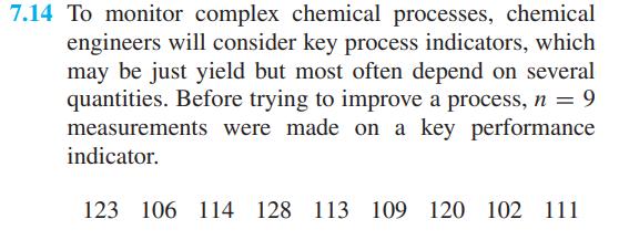
Use the data of Exercise 7.14 to estimate \(\sigma\) for the key performance indicator in terms of(a) the sample standard deviation;(b) the sample range.Compare the two estimates by expressing their difference as a percentage of the first.Data From Exercise 7.14 7.14 To monitor complex chemical
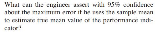
With reference to Example 7, Chapter 8, use the range of the second sample to estimate \(\sigma\) for the resiliency modulus of recycled materials from the second location. Compare the result with the standard deviation of the second sample.Data From Example 7 EXAMPLE 7 A two sample t test to show
Showing 5900 - 6000
of 7136
First
53
54
55
56
57
58
59
60
61
62
63
64
65
66
67
Last
Step by Step Answers