New Semester Started Get 50% OFF Study Help! --h --m --s Claim Now

Question Answers

Textbooks

Find textbooks, questions and answers

Oops, something went wrong!

Change your search query and then try again

Result Not Found

Books FREE
Study Help
Tutors
AI Study Planner NEW
Sell Books

Search
Sign In
Register

study help
business
introduction to probability statistics

Probability And Statistics For Engineers 9th Global Edition Richard Johnson, Irwin Miller, John Freund - Solutions

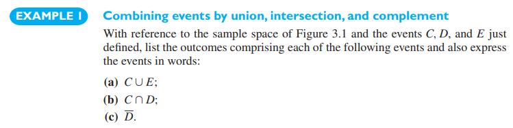
Verify that the function of Example 1 is, in fact, a probability density.Data From Example 1 EXAMPLE I Combining events by union, intersection, and complement With reference to the sample space of Figure 3.1 and the events C, D, and E just defined, list the outcomes comprising each of the following
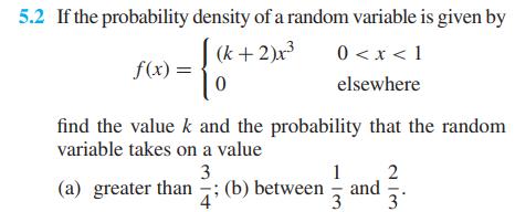
If the probability density of a random variable is given by\[f(x)= \begin{cases}(k+2) x^{3} & 0
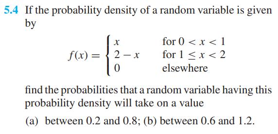
If the probability density of a random variable is given by\[f(x)= \begin{cases}x & \text { for } 0
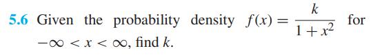
Given the probability density \(f(x)=\frac{k}{1+x^{2}}\) for \(-\infty
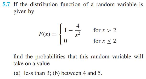
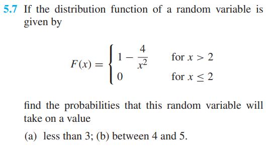
If the distribution function of a random variable is given by\[F(x)= \begin{cases}1-\frac{4}{x^{2}} & \text { for } x>2 \\ 0 & \text { for } x \leq 2\end{cases}\]find the probabilities that this random variable will take on a value(a) less than 3; (b) between 4 and 5 .
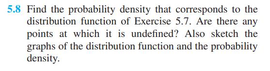
Find the probability density that corresponds to the distribution function of Exercise 5.7. Are there any points at which it is undefined? Also sketch the graphs of the distribution function and the probability density.Data From Exercise 5.7 5.7 If the distribution function of a random variable is
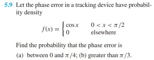
Let the phase error in a tracking device have probability density\[f(x)= \begin{cases}\cos x & 0
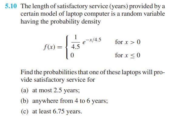
The length of satisfactory service (years) provided by a certain model of laptop computer is a random variable having the probability density\[f(x)= \begin{cases}\frac{1}{4.5} e^{-x / 4.5} & \text { for } x>0 \\ 0 & \text { for } x \leq 0\end{cases}\]Find the probabilities that one of these laptops
At a certain construction site, the daily requirement of gneiss (in metric tons) is a random variable having the probability density \[f(x)= \begin{cases}\frac{4}{81}(x+2)^{-(x+2) / 9} & \text { for } x>0 \\ 0 & \text { for } x \leq 0\end{cases}\]If the supplier's daily supply capacity is 25 metric
Prove that the identity \(\sigma^{2}=\mu_{2}^{\prime}-\mu^{2}\) holds for any probability density for which these moments exist.
Find \(\mu\) and \(\sigma^{2}\) for the probability density of Exercise 5.2.Data From Exercise 5.2 5.2 If the probability density of a random variable is given by (k+2)x f(x) = 0 0 < x < 1 elsewhere find the value k and the probability that the random variable takes on a value 3 1 2 (a) greater
Find \(\mu\) and \(\sigma^{2}\) for the probability density of Exercise 5.4.Data From Exercise 5.4 5.4 If the probability density of a random variable is given by X for 0 < x < 1 f(x) = 2-x for 1 < x
Find \(\mu\) and \(\sigma\) for the probability density obtained in Exercise 5.8.Data From Exercise 5.8Data From Exercise 5.7 5.8 Find the probability density that corresponds to the distribution function of Exercise 5.7. Are there any points at which it is undefined? Also sketch the graphs of the
Find \(\mu\) and \(\sigma\) for the distribution of the phase error of Exercise 5.9.Data From Exercise 5.9 5.9 Let the phase error in a tracking device have probabil- ity density f(x) = (9) = { o COS X 0
Find \(\mu\) for the distribution of the satisfactory service of Exercise 5.10.Data From Exercise 5.10 5.10 The length of satisfactory service (years) provided by a certain model of laptop computer is a random variable having the probability density 1 e-x/4.5 for x > 0 f(x) = 4.5 0 for x 0 Find the
Show that \(\mu_{2}^{\prime}\) and, hence, \(\sigma^{2}\) do not exist for the probability density of Exercise 5.6.Data From Exercise 5.6 5.6 Given the probability density f(x) = -
If a random variable has the standard normal distribution, find the probability that it will take on a value(a) less than 1.75 ;(b) less than -1.25 ;(c) greater than 2.06 ;(d) greater than -1.82 .
If a random variable has the standard normal distribution, find the probability that it will take on a value(a) between 0 and 2.3 ;(b) between 1.22 and 2.43 ;(c) between -1.45 and -0.45 ;(d) between -1.70 and 1.35 .
The nozzle of a mixing vibrator is tested for its number of vibrations. The vibration frequency, for each nozzle sample, can be modeled by a normal distribution with mean 128 and standard deviation 16 PdM.(a) If engineering specifications require the sample to have a vibration frequency of \(100
If a random variable has a normal distribution, what are the probabilities that it will take on a value within(a) 1 standard deviation of the mean;(b) 2 standard deviations of the mean;(c) 3 standard deviations of the mean;(d) 4 standard deviations of the mean?
Verify that(a) \(z_{0.005}=2.575\);(b) \(z_{0.025}=1.96\).
Given a random variable having the normal distribution with \(\mu=16.2\) and \(\sigma^{2}=1.5625\), find the probabilities that it will take on a value(a) greater than 16.8 ;(b) less than 14.9;(c) between 13.6 and 18.8 ;(d) between 16.5 and 16.7 .
The time for oil to percolate to all parts of an engine can be treated as a random variable having a normal distribution with mean 20 seconds. Find its standard deviation if the probability is 0.25 that it will take a value greater than 31.5 seconds.
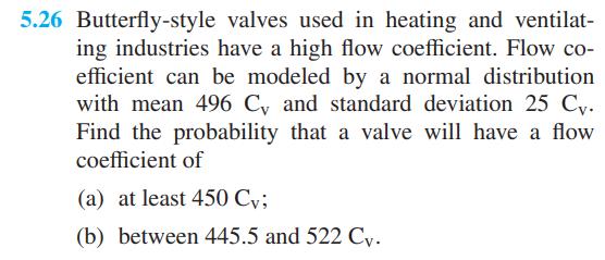
Butterfly-style valves used in heating and ventilating industries have a high flow coefficient. Flow coefficient can be modeled by a normal distribution with mean \(496 C_{V}\) and standard deviation \(25 C_{v}\). Find the probability that a valve will have a flow coefficient of(a) at least \(450
Refer to Exercise 5.26 but suppose that a large potential contract contains the specification that at most \(7.5 \%\) can have a flow coefficient less than \(420 \mathrm{C}_{\mathrm{v}}\). If the manufacturing process is improved to meet this specification, determine(a) the new mean \(\mu\) if the
Find the quartiles\[-z_{0.25} \quad z_{0.50} \quad z_{0.25}\]of the standard normal distribution.
The daily high temperature in a computer server room at the university can be modeled by a normal distribution with mean \(68.7^{\circ} \mathrm{F}\) and standard deviation \(1.2^{\circ} \mathrm{F}\). Find the probability that, on a given day, the high temperature will be(a) between 68.3 and
A machine produces soap bars with a weight of \(80 \pm\) \(0.10 \mathrm{~g}\). If the weight of the soap bars manufactured by the machine may be looked upon as a random variable having normal distribution with \(\mu=80.05 \mathrm{~g}\) and \(\sigma=0.05 \mathrm{~g}\), what percentage of these bars
The number of teeth of a \(12 \%\) tooth gear produced by a machine follows a normal distribution. Verify that if \(\sigma=1.5\) and the mean number of teeth is \(13,74 \%\) of the gears contain at least 12 teeth.
The quantity of aerated water that a machine puts in a bottle of a carbonated beverage follows a normal distribution with a standard deviation of \(0.25 \mathrm{~g}\). At what "normal" (mean) weight should the machine be set so that no more than \(8 \%\) of the bottles have more than \(20
An automatic machine fills distilled water in \(500-\mathrm{ml}\) bottles. Actual volumes are normally distributed about a mean of \(500 \mathrm{ml}\) and their standard deviation is \(20 \mathrm{ml}\)(a) What proportion of the bottles are filled with water outside the tolerance limit of \(475
If a random variable has the binomial distribution with \(n=25\) and \(p=0.65\), use the normal approximation to determine the probabilities that it will take on(a) the value 15 ;(b) a value less than 10 .
From past experience, a company knows that, on average, \(5 \%\) of their concrete does not meet standards. Use the normal approximation of the binomial distribution to determine the probability that among 2000 bags of concrete, 75 bags contain concrete that does not meet standards.
The probability that an electronic component will fail in less than 1,000 hours of continuous use is 0.25 . Use the normal approximation to find the probability that among 200 such components fewer than 45 will fail in less than 1,000 hours of continuous use.
Workers in silicon factories are prone to a lung disease called silicosis. In a recent survey in a factory, about \(11 \%\) of the workers have been infected by it. Assume the same rate of infection holds everywhere. Use the normal distribution to approximate the probability that, out of a random
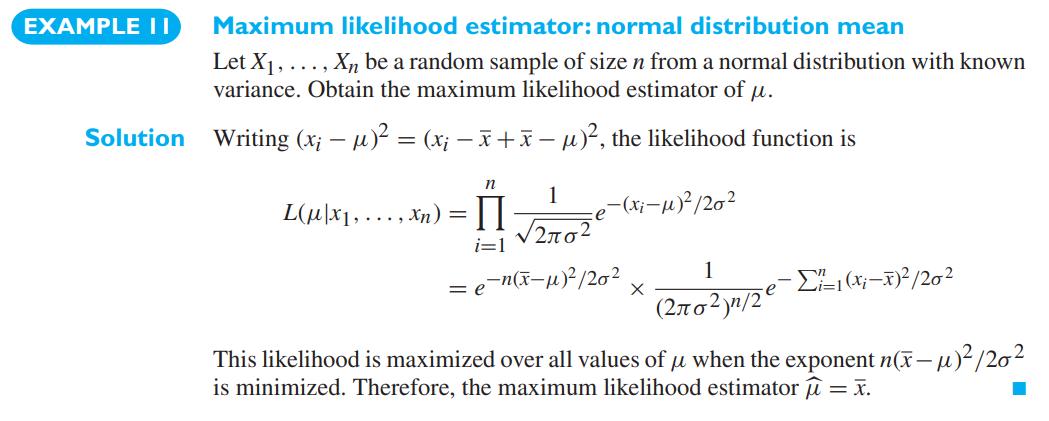
Refer to Example 11 concerning the experiment that confirms electron antineutrinos change type. Suppose instead that there are 400 electron antineutrinos leaving the reactor. Repeat parts (a)-(c) of the example.Data From Example 11 EXAMPLE II Maximum likelihood estimator: normal distribution mean
To illustrate the law of large numbers mentioned on Page 116, find the probabilities that the proportion of drawing a club from a fair deck of cards will be anywhere from 0.24 to 0.26 when a card is drawn(a) 100 times;(b) 10,000 times. EXAMPLE 20 Chebyshev's theorem with a large number of Bernoulli
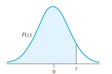
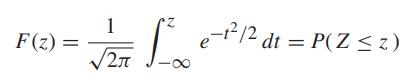
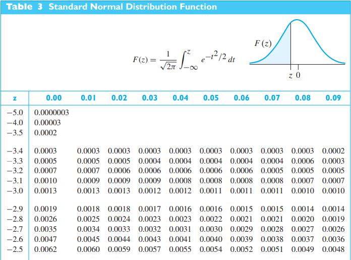
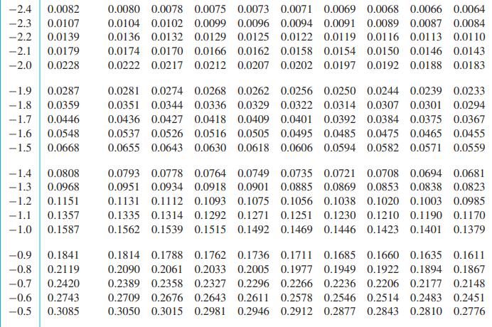
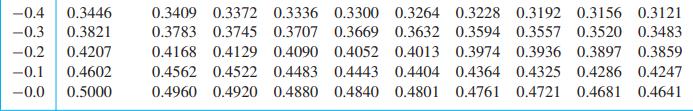
Verify the identity \(F(-z)=1-F(z)\) given on page 141. F(z) 0 N
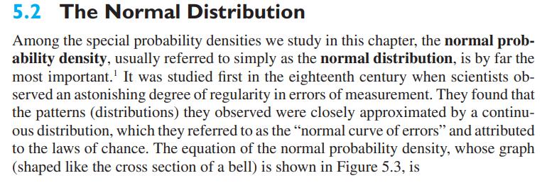
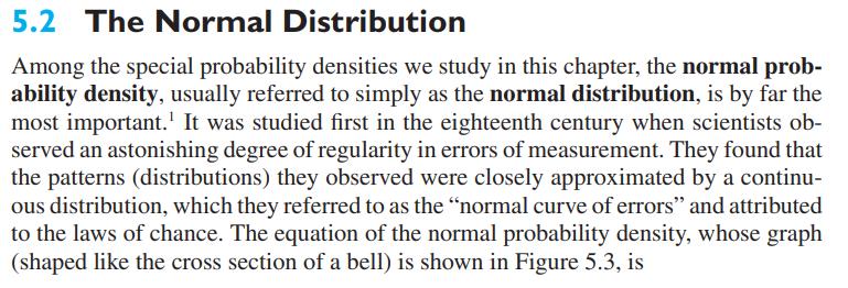
Verify that the parameter \(\mu\) in the expression for the normal density on page 140 , is, in fact, its mean. 5.2 The Normal Distribution Among the special probability densities we study in this chapter, the normal prob- ability density, usually referred to simply as the normal distribution, is
Verify that the parameter \(\sigma^{2}\) in the expression for the normal density on page 140 is, in fact, its variance. 5.2 The Normal Distribution Among the special probability densities we study in this chapter, the normal prob- ability density, usually referred to simply as the normal
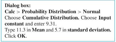
Normal probabilities can be calculated using MINITAB. Let \(X\) have a normal distribution with mean 11.3 and standard deviation 5.7. The following steps yield the cumulative probability of 9.31 or smaller, or \(P(X \leq 9.31)\).Output: Normal with mean \(=11.3000\) and standard deviation
Find the distribution function of a random variable having a uniform distribution on \((0,1)\).
In a manufacturing process, the error made in determining the composition of an alloy is a random variable having the uniform density with \(\alpha=-0.075\) and \(\beta=0.010\). What are the probabilities that such an error will be(a) between 0.050 and 0.001 ?(b) between 0.001 and 0.008 ?
From experience Mr. Harris has found that the low bid on a construction job can be regarded as a random variable having the uniform density\[f(x)= \begin{cases}\frac{3}{4 C} & \text { for } \frac{2 C}{3}
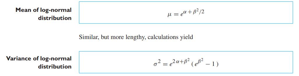
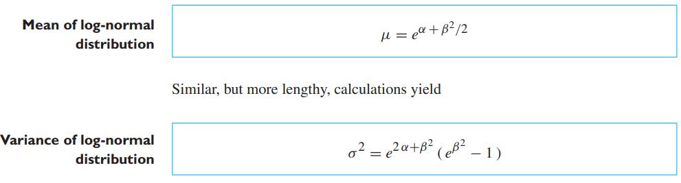
Verify the expression given on page 154 for the mean of the log-normal distribution. Mean of log-normal distribution M = ea+B 12 Variance of log-normal Similar, but more lengthy, calculations yield distribution (eB2 -1)
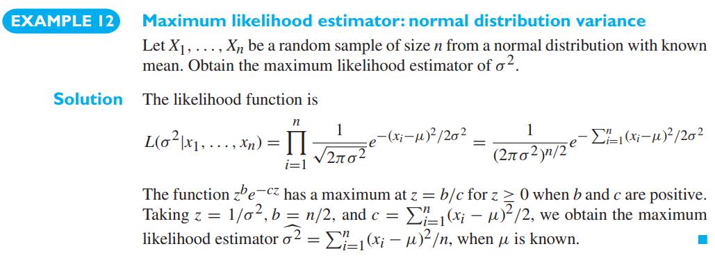
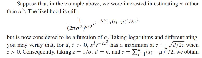
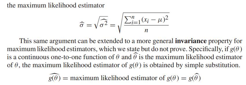
With reference to the Example 12, find the probability that \(I_{o} / I_{i}\) will take on a value between 7.0 and 7.5.Data From Example 12 EXAMPLE 12 Maximum likelihood estimator: normal distribution variance Let X1, ..., Xn be a random sample of size n from a normal distribution with known mean.
If a random variable has the log-normal distribution with \(\alpha=-3\) and \(\beta=3\), find its mean and its standard deviation.
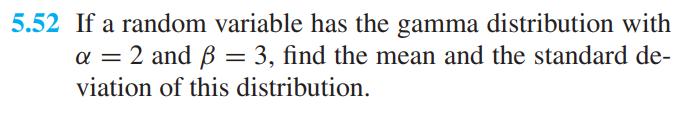
If a random variable has the gamma distribution with \(\alpha=2\) and \(\beta=3\), find the mean and the standard deviation of this distribution.
With reference to Exercise 5.52, find the probability that the random variable will take on a value less than 5.Data From Exercise 5.52 5.52 If a random variable has the gamma distribution with = 2 and B = 3, find the mean and the standard de- viation of this distribution.
At a construction site, the daily requirement of gneiss (in metric tons) is a random variable having a gamma distribution with \(\alpha=2\) and \(\beta=5\). If their supplier's daily supply capacity is 25 metric tons, what is the probability that this capacity will be inadequate on any given day?
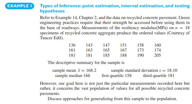
With reference to the Example 14, suppose the expert opinion is in error. Calculate the probability that the supports will survive if(a) \(\mu=3.0\) and \(\sigma^{2}=0.09\);(b) \(\mu=4.0\) and \(\sigma^{2}=0.25\).Data From Example 14 EXAMPLE I Types of Inference: point estimation, interval
Verify the expression for the variance of the gamma distribution given on page 156 . Mean of log-normal distribution M = ea+B 12 Variance of log-normal Similar, but more lengthy, calculations yield distribution = (eB2 1)
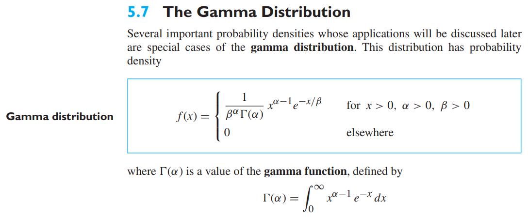
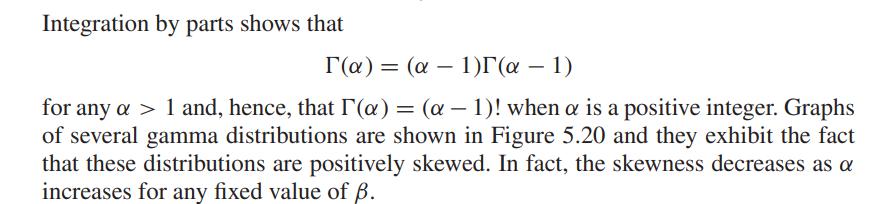
Show that when \(\alpha>1\), the graph of the gamma density has a relative maximum at \(x=\beta(\alpha-1)\). What happens when \(0
The server of a multinational corporate network can run for an amount of time without having to be rebooted and this amount of time is a random variable having the exponential distribution \(\beta=30\) days. Find the probabilities that such a server will(a) have to be rebooted in less than 10
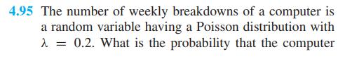
With reference to Exercise 4.95, find the percent of the time that the interval between breakdowns of the computer will be(a) less than 1 week;(b) at least 5 weeks.Data From Exercise 4.95 4.95 The number of weekly breakdowns of a computer is a random variable having a Poisson distribution with
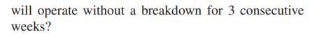
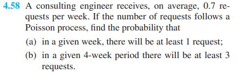
With reference to Exercise 4.58, find the probabilities that the time between successive requests for consulting will be(a) less than 0.5 week;(b) more than 3 weeks.Data From Exercise 4.58 4.58 A consulting engineer receives, on average, 0.7 re- quests per week. If the number of requests follows a
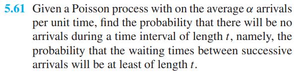
Given a Poisson process with on the average \(\alpha\) arrivals per unit time, find the probability that there will be no arrivals during a time interval of length \(t\), namely, the probability that the waiting times between successive arrivals will be at least of length \(t\).
Use the result of Exercise 5.61 to find an expression for the probability density of the waiting time between successive arrivals.Data From Exercise 5.61 5.61 Given a Poisson process with on the average arrivals per unit time, find the probability that there will be no arrivals during a time
Verify for \(\alpha=3\) and \(\beta=3\) that the integral of the beta density, from 0 to 1 , is equal to 1 .
If the ratio of defective switches produced during complete production cycles in the previous month can be looked upon as a random variable having a beta distribution with \(\alpha=3\) and \(\beta=6\), what is the probability that in any given year, there will be fewer than \(5 \%\) defective
Suppose the proportion of error in code developed by a programmer, which varies from software to software, may be looked upon as a random variable having the beta distribution with \(\alpha=2\) and \(\beta=7\).(a) Find the mean of this beta distribution, namely, the average proportion of errors in
Show that when \(\alpha>1\) and \(\beta>1\), the beta density has a relative maximum at\[x=\frac{\alpha-1}{\alpha+\beta-2}\]
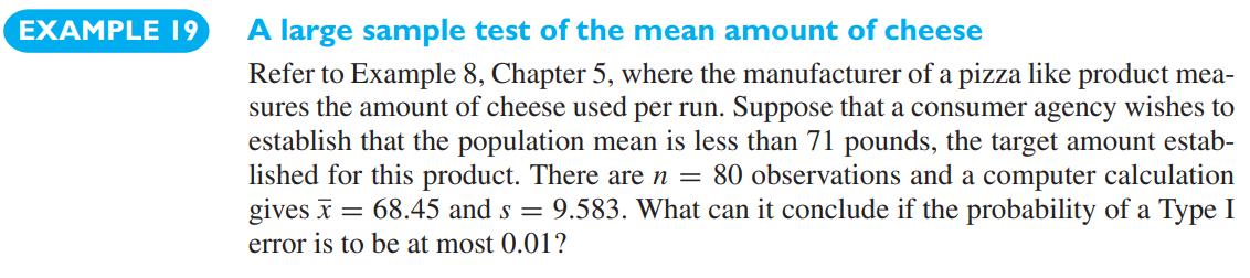
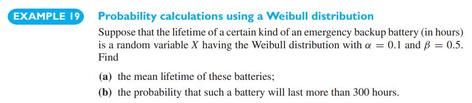
With reference to the Example 19, find the probability that such a battery will not last 100 hours.Data From Example 19 EXAMPLE 19 A large sample test of the mean amount of cheese Refer to Example 8, Chapter 5, where the manufacturer of a pizza like product mea- sures the amount of cheese used per
Suppose that the time to failure (in minutes) of certain electronic components subjected to continuous vibrations may be looked upon as a random variable having the Weibull distribution with \(\alpha=\frac{1}{5}\) and \(\beta=\frac{1}{3}\).(a) How long can such a component be expected to last?(b)
Suppose that the processing speed (in milliseconds) of a supercomputer is a random variable having the Weibull distribution with \(\alpha=0.005\) and \(\beta=0.125\). What is the probability that such a supercomputer will have similar processing speeds after running for \(50,000 \mathrm{~ms}\) ?
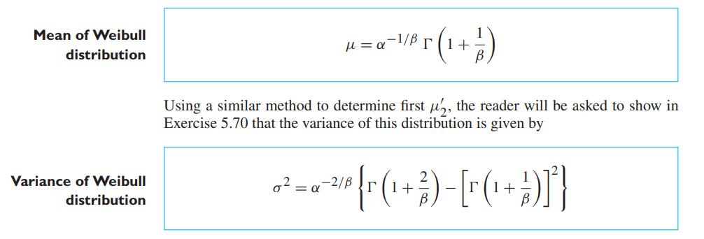
Verify the formula for the variance of the Weibull distribution given on page 160. Mean of Weibull distribution Variance of Weibull distribution + Using a similar method to determine first 2, the reader will be asked to show in Exercise 5.70 that the variance of this distribution is given by -2/B
Two transistors are needed for an integrated circuit. Of the eight available, three have broken insulation layers, two have poor diodes, and three are in good condition. Two transistors are selected at random.(a) Find the joint probability distribution of \(X_{1}=\) the number of transistors with
Two random variables are independent and each has a binomial distribution with success probability 0.7 and 4 trials.(a) Find the joint probability distribution.(b) Find the probability that the first random variable is greater than the second.
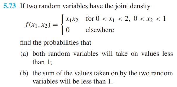
If two random variables have the joint density\[f\left(x_{1}, x_{2}\right)= \begin{cases}x_{1} x_{2} & \text { for } 0
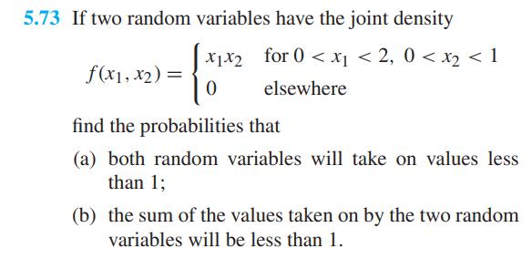
With reference to Exercise 5.73, find the joint cumulative distribution function of the two random variables, the cumulative distribution functions of the individual random variables, and check whether the two random variables are independent.Data From Exercise 5.73 5.73 If two random variables
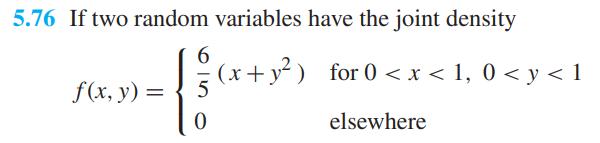
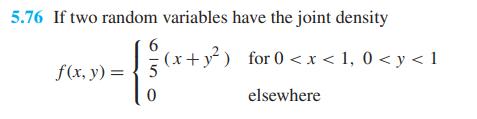
If two random variables have the joint density \(f(x, y)= \begin{cases}\frac{6}{5}\left(x+y^{2}\right) & \text { for } 0
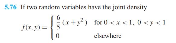
With reference to Exercise 5.76, find both marginal densities and use them to find the probabilities that(a) \(X>0.8\);(b) \(YData From Exercise 5.76 5.76 If two random variables have the joint density f(x, y) = = 6 0 (x + y) for 0 < x < 1, 0 < y < 1 elsewhere
With reference to Exercise 5.76, find(a) an expression for \(f_{1}(x \mid y)\) for \(0(b) an expression for \(f_{1}(x \mid 0.5)\);(c) the mean of the conditional density of the first random variable when the second takes on the value 0.5 .Data From Exercise 5.76 5.76 If two random variables have
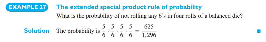
With reference to Example 27, find expressions for(a) the conditional density of the first random variable when the second takes on the value \(x_{2}=0.25\);(b) the conditional density of the second random variable when the first takes on the value \(x_{1}\).Data From Example 27 EXAMPLE 27 The
If three random variables have the joint density\[f(x, y, z)=\left\{\begin{array}{lc}k(x+y) e^{-z} & \text { for } 0
A precision drill positioned over a target point will make an acceptable hole if it is within 5 microns of the target. Using the target as the origin of a rectangular system of coordinates, assume that the coordinates \((x, y)\) of the point of contact are values of a pair of random variables
with \(\mu_{1}=\mu_{2}=0\) and \(\sigma=2\). What is the probability that the hole will be acceptable?
With reference to Exercise 5.73, find the expected value of the random variable whose values are given by \(g\left(x_{1}, x_{2}\right)=x_{1}+x_{2}\).Data From Exercise 5.73 5.73 If two random variables have the joint density x1x2 for 0 < x1 < 2, 0 < x < 1 f(x1, x2)= 0 elsewhere find the
With reference to Exercise 5.76, find the expected value of the random variable whose values are given by \(g(x, y)=x^{2} y\).Data From Exercise 5.76 5.76 If two random variables have the joint density 6 f(x, y) = (x+y) for 0 < x < 1, 0 < y < 1 5 0 elsewhere
If measurements of the length and the width of a rectangle have the joint density\[f(x, y)=\left\{\begin{array}{cc}\frac{1}{a b} & \text { for } L-\frac{a}{2}
Establish a relationship between \(f_{1}\left(x_{1} \mid x_{2}\right)\), \(f_{2}\left(x_{2} \mid x_{1}\right), f_{1}\left(x_{1}\right)\), and \(f_{2}\left(x_{2}\right)\).
If \(X_{1}\) has mean 1 and variance 5 while \(X_{2}\) has mean - 1 and variance 5 , and the two are independent, find(a) \(E\left(X_{1}+X_{2}\right)\);(b) \(\operatorname{Var}\left(X_{1}+X_{2}\right)\).
If \(X_{1}\) has mean 8 and variance 2 while \(X_{2}\) has mean -12.5 and variance 2.25 , and the two are independent, find(a) \(E\left(X_{1}-X_{2}\right)\);(b) \(\operatorname{Var}\left(X_{1}-X_{2}\right)\).
If \(X_{1}\) has mean 1 and variance 3 while \(X_{2}\) has mean -2 and variance 5 , and the two are independent, find(a) \(E\left(X_{1}+2 X_{2}-3\right)\)(b) \(\operatorname{Var}\left(X_{1}+2 X_{2}-3\right)\).
The time taken by a traditional nuclear reactor to generate one nuclear chain reaction with fast neutrons, \(X_{1}\), has mean 10 nanoseconds and variance 4 , while the time taken by an improved design of the reactor, \(X_{2}\), has mean 8 nanoseconds and variance 2.5. Find the expected time
Let \(X_{1}, X_{2}, \ldots, X_{20}\) be independent and let each have the same marginal distribution with mean 10 and variance 3. Find(a) \(E\left(X_{1}+X_{2}+\cdots+X_{20}\right)\);(b) \(\operatorname{Var}\left(X_{1}+X_{2}+\cdots+X_{20}\right)\).
Let \(f(x)=0.2\) for \(x=0,1,2,3,4\).(a) Find the moment generating function.(b) Obtain \(E(X)\) and \(E\left(X^{2}\right)\) by differentiating the moment generating function.
Let\[f(x)=0.40\left(\begin{array}{l}4 \\x\end{array}\right) \quad \text { for } x=0,1,2,3,4\](a) Find the moment generating function.(b) Obtain \(E(X)\) and \(E\left(X^{2}\right)\) by differentiating the moment generating function.
Let \(Z\) have a normal distribution with mean 0 and variance 1 .(a) Find the moment generating function of \(Z^{2}\).(b) Identify the distribution of \(Z^{2}\) by recognizing the form of the moment generating function.
Let \(X\) be a continuous random variable having probability density function\[f(x)= \begin{cases}2 e^{-2 x} & \text { for } x>0 \\ 0 & \text { elsewhere }\end{cases}\](a) Find the moment generating function.(b) Obtain \(E(X)\) and \(E\left(X^{2}\right)\) by differentiating the moment generating
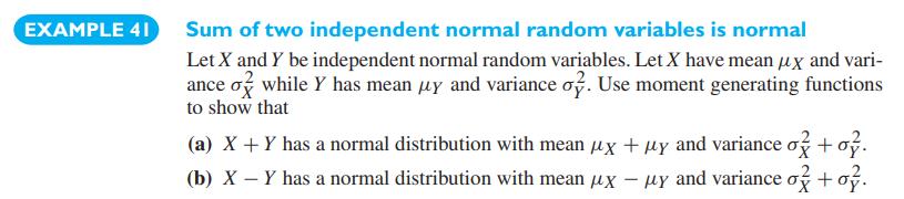
Establish the result in Example 41 concerning the difference of two independent normal random variables, \(X\) and \(Y\).Data From Example 41 EXAMPLE 41 Sum of two independent normal random variables is normal Let X and Y be independent normal random variables. Let X have mean x and vari- ance of
Let \(X\) and \(Y\) be independent normal random variables with\[\begin{array}{lll}E(X)=4 & \text { and } & \sigma_{X}^{2}=25 \\E(Y)=3 & \text { and } & \sigma_{Y}^{2}=16\end{array}\](a) Use moment generating functions to show that \(5 X-4 Y+7\) has a normal distribution.(b) Find the mean and
Let \(X\) have the geometric distribution\[f(x)=p(1-p)^{x-1} \quad \text { for } x=1,2, \ldots\](a) Obtain the moment generating function for\[t
For any 11 observations,(a) Use software or Table 3 to verify the normal scores \(-1.38-0.97-0.67-0.43-0.21 \quad 0 \quad 0.210 .430 .670 .971 .38\)(b) Construct a normal scores plot using the observations on the times between neutrinos in Exercise 2.7.Data From Table 3Data From Exercise 2.7 Table
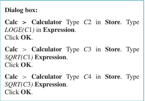
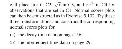
(Transformations) The MINITAB commands Dialog box: Calc Calculator Type C2 in Store. Type LOGE(C1) in Expression. Click OK. Calc Calculator Type C3 in Store. Type SQRT(C1) Expression. Click OK. Calc Calculator Type C4 in Store. Type SQRT(C3) Expression. Click OK.
Verify that(a) the exponential density \(0.3 e^{-0.3 x}, x>0\) corresponds to the distribution function \(F(x)=\) \(1-e^{-0.3 x}, x>0\)(b) the solution of \(u=F(x)\) is given by \(x=\) \([-\ln (1-u)] / 0.3\).
Verify that(a) the Weibull density \(\alpha \beta x^{\beta-1} e^{-a x^{\beta}}, x>0\), corresponds to the distribution function \(F(x)=\) \(1-e^{-a x^{\beta}}, x>0\)(b) the solution of \(u=F(x)\) is given by \(x=\) \(\left[-\frac{1}{\alpha} \ln (1-u)\right]^{1 / \beta}\).
Consider two independent standard normal variables whose joint probability density is\[\frac{1}{2 \pi} e^{-\left(z_{1}^{2}+z_{2}^{2}\right) / 2}\]Under a change to polar coordinates, \(z_{1}=\) \(r \cos (\theta), z_{2}=r \sin (\theta)\), we have \(r^{2}=z_{1}^{2}+z_{2}^{2}\) and \(d z_{1} d z_{2}=r
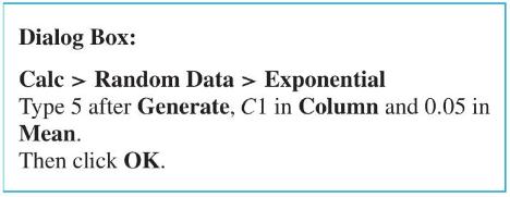
The statistical package MINITAB has a random number generator. To simulate 5 values from an exponential distribution having mean \(\beta=0.05\), chooseOutput:One call produced the output \(\begin{array}{lllll}0.031949 & 0.004643 & 0.030029 & 0.112834 & 0.064642\end{array}\)Generate
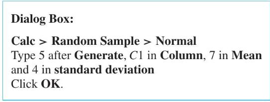
The statistical package MINITAB has a normal random number generator. To simulate 5 values from a normal distribution having mean 7 and standard deviation 4, and place them in \(\mathrm{C}\), use the commandsOutput:One call produced the output \[\begin{array}{lllll}5.42137 & 6.98061 &

Showing 6200 - 6300 of 7136

First
56
57
58
59
60
61
62
63
64
65
66
67
68
69
70
Last

Step by Step Answers

Services

Sitemap
Fun
Definitions
Become Tutor
Used Textbooks
Study Help Categories
Recent Questions
Expert Questions
Campus Wear
Sell Your Books

Company Info

Security
Copyrights
Privacy Policy
Terms & Conditions
SolutionInn Fee
Scholarship
Online Quiz
Give Feedback, Get Rewards

Get In Touch

About Us
Contact Us
Career
Jobs
FAQ
Student Discount
Campus Ambassador

Secure Payment

Download Our App

© 2026 SolutionInn. All Rights Reserved