New Semester
Started
Get
50% OFF
Study Help!
--h --m --s
Claim Now
Question Answers
Textbooks
Find textbooks, questions and answers
Oops, something went wrong!
Change your search query and then try again
S
Books
FREE
Study Help
Expert Questions
Accounting
General Management
Mathematics
Finance
Organizational Behaviour
Law
Physics
Operating System
Management Leadership
Sociology
Programming
Marketing
Database
Computer Network
Economics
Textbooks Solutions
Accounting
Managerial Accounting
Management Leadership
Cost Accounting
Statistics
Business Law
Corporate Finance
Finance
Economics
Auditing
Tutors
Online Tutors
Find a Tutor
Hire a Tutor
Become a Tutor
AI Tutor
AI Study Planner
NEW
Sell Books
Search
Search
Sign In
Register
study help
business
introduction to probability statistics
Introduction To Probability Statistics And Random Processes 1st Edition Hossein Pishro-Nik - Solutions
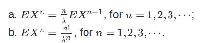
Let X ∼ Exponential(λ). Show that
Let X ∼ Uniform(−1, 1) and Y = X2. Find the CDF and PDF of Y.
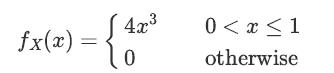
Let X be a continuous random variable with PDFand let Y = 1/X. Find fY (y). 1={1,2² 4x³ 0 fx(x) 0 < x < 1 otherwise
Let X ∼ N(3, 9).a. Find P(X > 0).b. Find P(−3 < X < 8).c. Find P(X > 5|X > 3).
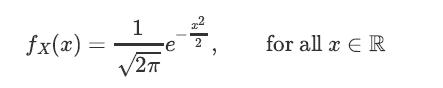
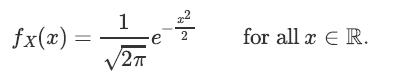
Let X be a continuous random variable with PDFand let Y = X2. Find fY(y). fx(x) = 1 2πT for all x ER
Let X ∼ N(3, 9) and Y = 5 −X.a. Find P(X > 2).b. Find P(−1 < Y < 3).c. Find P(X > 4|Y < 2).
Let X be a continuous random variable with PDFand let Y =√|X̄|. Find fY(y). 1 fx(x) = e /27 for all x E R.
Let X ∼ N(−5, 4).a. Find P(X < 0).b. Find P(−7 < X < −3).c. Find P(X > −3|X > −5).
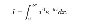
Answer the following questions:1. Find Γ(7/2).2. Find the value of the following integral: T = 1 * I 2°e52dư.
Let X ∼ Exponential(2) and Y = 2 +3X.a. Find P(X > 2).b. Find EY and V ar(Y ).c. Find P(X > 2|Y < 11).
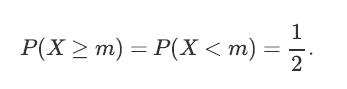
The median of a continuous random variable X can be defined as the unique real number m that satisfiesFind the median of the following random variablesa. X ∼ Uniform(a, b).b. Y ∼ Exponential(λ).c. W ∼ N(μ,σ2). P(X ≥ m) = P(X
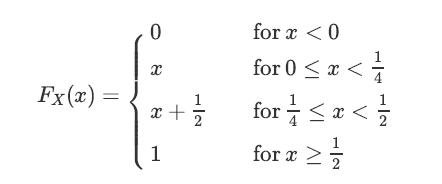
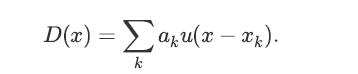
Let X be a random variable with the following CDFa. Plot FX(x) and explain why X is a mixed random variable.b. Find P(X ≤ 1/3).c. Find P(X ≥ 1/4).d. Write CDF of X in the form of FX(x) = C(x) +D(x), where C(x) is a continuous function and D(x) is in the form of a staircase function, i.e.,e.
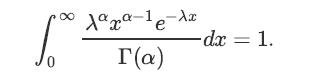
Using the properties of the gamma function, show that the gamma PDF integrates to 1, i.e., show that for α,λ > 0, we have ∞ Xªxª-¹e-λx е r(a) So dx = 1.
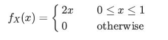
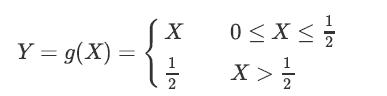
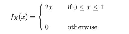
Let X be a continuous random variable with the following PDF:Let alsoFind the CDF of Y. fx(x) 2x 0 0 ≤ x ≤ 1 otherwise
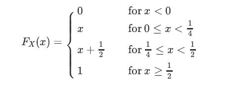
Let X be a random variable with the following CDFa. Find the generalized PDF of X, fX(x).b. Find EX using fX(x).c. Find V ar(X) using fX(x). Fx(x) = 0 8 x + 1 2 for x < 0 for 0 < x 1
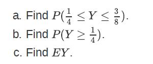
Let Y be the mixed random variable defined in Example 4.14.Example 4.14:Let X be a continuous random variable with the following PDF:Let alsoFind the CDF of Y. a. Find P(≤Y ≤). b. Find P(Y>¹). c. Find EY.
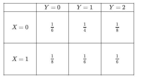
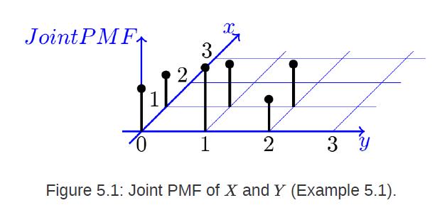
Consider two random variables X and Y with joint PMF given in Table 5.1.Figure 5.1 shows PXY (x, y).a. Find P(X = 0,Y ≤ 1).b. Find the marginal PMFs of X and Y .c. Find P(Y = 1|X = 0).d. Are X and Y independent? X = 0 X = 1 Y = 0 Y = 1 H Y = 2 6
A surveillance system is in charge of detecting intruders to a facility. There are two hypotheses to choose from:H0: No intruder is present.H1: There is an intruder.The system sends an alarm message if it accepts H1. Suppose that after processing the data, we obtain P(H1|y) = 0.05. Also, assume
Let X ∼ Bernoulli(p) and Y ∼ Bernoulli(q) be independent, where 0 < p, q < 1. Find the joint PMF and joint CDF for X and Y .
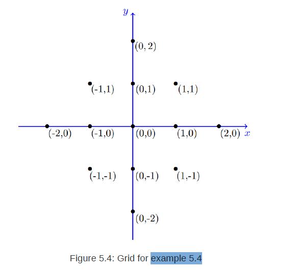
Let X and Y be the same as in Example 5.4.a. Find E[X|Y = 1|.b. Find E[X|−1c. Find E[|X||−1Example 5.4:Consider the set of points in the grid shown in Figure 5.4. These are the points in set G defined asSuppose that we pick a point (X,Y ) from this grid completely at random. Thus, each point
Let X and Y be two independent Geometric(p) random variables. Find E X²+Y2- XY
I roll a fair die. Let X be the observed number. Find the conditional PMF of X given that we know the observed number was less than 5.
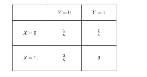
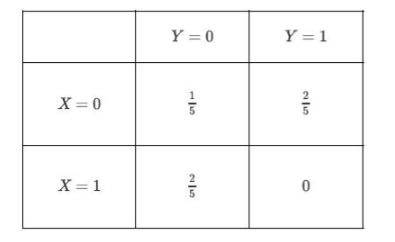
Consider two random variables X and Y with joint PMF given in Table 5.2. Let Z = E[X|Y].a. Find the Marginal PMFs of X and Y .b. Find the conditional PMF of X given Y = 0 and Y = 1, i.e., find PX|Y (x|0) and PX|Y (x|1).c. Find the PMF of Z.d. Find EZ, and check that EZ = EX.e. Find Var(Z). X =
Let X, Y, and Z = E[X|Y] be as in Example 5.11. Let also V =Var(X|Y).a. Find the PMF of V .b. Find EV.c. Check that Var(X) = E(V )+Var(Z).Example 5.11:Consider two random variables X and Y with joint PMF given in Table 5.2. Let Z = E[X|Y]. X = 0 X=1 Y = 0 16 25 Y=1 235 0
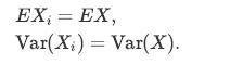
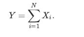
Let N be the number of customers that visit a certain store in a given day. Suppose that we know E[N] and Var(N). Let Xi be the amount that the ith customer spends on average. We assume Xi's are independent of each other and also independent of N. We further assume they have the same mean and
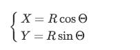
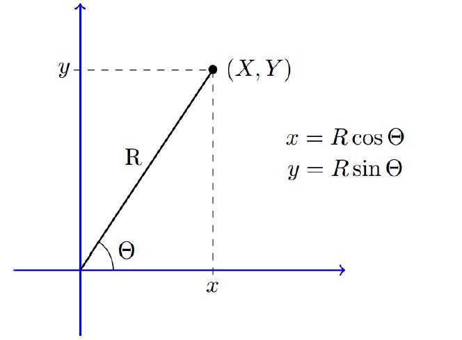
In Problem 29, suppose that X and Y are independent Uniform(0, 1) random variables. Find the joint PDF of R and Θ. Are R and Θ independent?Problem 29Let X and Y be two independent standard normal random variables. Consider the point (X, Y) in the x − y plane. Let (R,Θ) be the corresponding
Let X and Y be two independent standard normal random variables. Consider the point (X,Y ) in the x −y plane. Let (R,Θ) be the corresponding polar coordinates as shown in Figure 5.11. The inverse transformation is given bywhere, R ≥ 0 and −π X = R cos Ⓒ Y = Rsin Ⓒ
Let X and Y be two independent Uniform(0, 1) random variables. Find FXY (x, y).
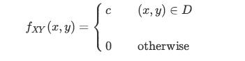
Let X and Y be as in Example 5.24 in Section 5.2.3, i.e., suppose that we choose a point (X,Y ) uniformly at random in the unit disc Are X and Y uncorrelated?Example 5.24 in Section 5.2.3Consider the unit disc D = {(x, y)|x2 +y2 ≤ 1}.Suppose that we choose a point (X,Y ) uniformly at random in
Let X and Y be two random variables with joint PDF fXY (x, y). Let Z = X +Y . Find fZ(z).
If Y ∼ Uniform(0, 1), find E[Yk] using MY(s).
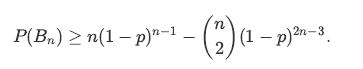
Let Bn be the event that a graph randomly generated according to G(n, p) model has at least one isolated node. Show that P(Bn) > n(1-p)"-1. (2) (1 (1-p) 2-3
If X ∼ Binomial(n, p) find the MGF of X.
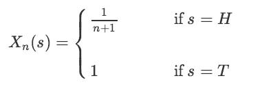
Consider the following random experiment: A fair coin is tossed once. Here, the sample space has only two elements S = {H,T}. We define a sequence of random variables X1, X2, X3, ⋯ on this sample space as follows:a. Are the Xi's independent?b. Find the PMF and CDF of Xn, FXn(x) for n = 1, 2,
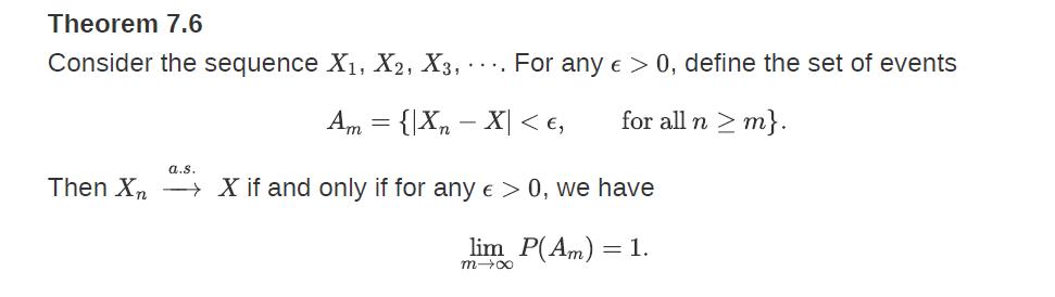
Let X1, X2, X3, ⋯ be independent random variables, where Xn ∼ Bernoulli (1 n) for n = 2, 3,⋯. The goal here is to check whether Xn a.s.→ 0.1. Check that2. Show that the sequence X1, X2, . . . does not converge to 0 almost surely using Theorem 7.6 ∞ Σx=₁ P(|X₂| > €) = ∞. n=1
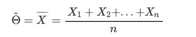
Let X1, X2, X3, . . ., Xn be a random sample. Show that the sample meanis an unbiased estimator of θ = EXi. Ô=X = X₁ + X₂+...+Xn n
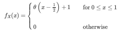
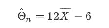
Let X1, X2, X3, . . ., Xn be a random sample from the following distributionwhere θ ∈ [−2, 2] is an unknown parameter. We define the estimator ^Θn asto estimate θ.a. Is ^Θn an unbiased estimator of θ?b. Is ^Θn a consistent estimator of θ?c. Find the mean squared error (MSE) of ^Θn.
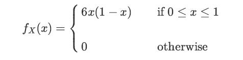
Let X be a continuous random variable with the following PDFSuppose that we knowFind the posterior density of X given Y = 2, fX|Y (x|2). fx(x) = 6x(1-x) 0 if 0 ≤ x ≤ 1 otherwise
For the following random samples, find the maximum likelihood estimate of θ:1. Xi ∼ Binomial(3, θ), and we have observed (x1,x2,x3,x4) = (1, 3, 2, 2).2. Xi ∼ Exponential(θ) and we have observed (x1,x2,x3,x4) = (1.23, 3.32, 1.98, 2.12).
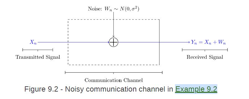
Consider a communication channel as shown in Figure 9.2. We can model the communication over this channel as follows. At time n, a random variable Xn is generated and is transmitted over the channel. However, the channel is noisy. Thus, at the receiver, a noisy version of Xn is received. More
Suppose that you would like to estimate the portion of voters in your town that plan to vote for Party A in an upcoming election. To do so, you take a random sample of size n from the likely voters in the town. Since you have a limited amount of time and resources, your sample is relatively small.
Let X be a continuous random variable with the following PDFAlso, suppose thatFind the MAP estimate of X given Y = 5. fx(x) = 3x² 0 if 0 ≤ x ≤ 1 otherwise
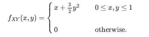
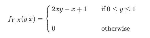
Let X and Y be two jointly continuous random variables with joint PDFFind the MAP and the ML estimates of X given Y = y. fxy(x, y) = x+2y² 0 0≤x, y ≤ 1 otherwise.
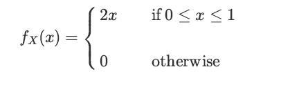
Let X be a continuous random variable with the following PDF:Also, suppose thatFind the MAP estimate of X given Y = 3. fx(x) = 2x { 0 if 0 ≤ x ≤ 1 otherwise
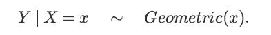
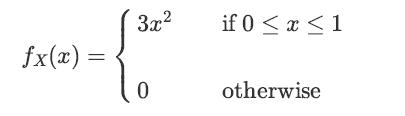
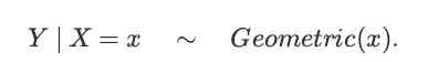
Let X ∼ Uniform(0, 1). Suppose that we know Y | X = x ∼ Geometric(x).Find the posterior density of X given Y = 2, fX|Y (x|2).
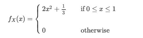
Let X be a continuous random variable with the following PDFWe also know thatFind the MMSE estimate of X, given Y = y is observed. fx(x) = 2x² + 0 3 if 0 ≤ x ≤ 1 otherwise
Let X ∼ N(0, 1) andwhere W ∼ N(0, 1) is independent of X.a. Find the MMSE estimator of X given Y , ( X̂M).b. Find the MSE of this estimator, using MSE = E[(X −X̂M)2].c. Check that E[X2] = E[ X̂2M]+E[X̃2]. Y = 2X + W,
Suppose that the signal X ∼ N(0,σ2X) is transmitted over a communication channel. Assume that the received signal is given by Y = X +W, where W ∼ N(0,σ2W) is independent of X.1. Find the ML estimate of X, given Y = y is observed.2. Find the MAP estimate of X, given Y = y is observed.
Let X be a continuous random variable with the following PDFWe also know thatFind the MMSE estimate of X, given Y = y is observed. fx(x) = 2x 0 if 0 ≤ x ≤ 1 otherwise
Suppose X ∼ Uniform(0, 1), and given X = x, Y ∼ Exponential (λ = 1/2x).a. Find the linear MMSE estimate of X given Y .b. Find the MSE of this estimator.c. Check that E[X̃Y ] = 0.
Suppose that the signal X ∼ N(0,σ2X) is transmitted over a communication channel.Assume that the received signal is given by Y = X +W, where W ∼ N(0,σ2W) is independent of X.a. Find the MMSE estimator of X given Y , ( X̂M).b. Find the MSE of this estimator.
Let X ∼ N(0, 1) and Y = X +W, where W ∼ N(0, 1) is independent of X.a. Find the MMSE estimator of X given Y , ( X̂M).b. Find the MSE of this estimator, using MSE = E[(X −X̂M)2].c. Check that E[X2] = E[ X̂2M] + E[X̃2].
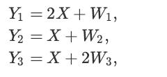
Let X be an unobserved random variable with EX = 0, Var(X) = 5. Assume that we have observed Y1 and Y2 given byY1 = 2X +W1,Y2 = X +W2,where EW1 = EW2 = 0, Var(W1) = 2, and Var(W2) = 5. Assume that W1, W2 , and X are independent random variables. Find the linear MMSE estimator of X, given Y1 and Y2.
Consider again Problem 8, in which X is an unobserved random variable with EX = 0, Var(X) = 5. Assume that we have observed Y1 and Y2 given byY1 = 2X +W1,Y2 = X +W2,where EW1 = EW2 = 0, Var(W1) = 2, and Var(W2) = 5. Assume that W1, W2 , and X are independent random variables. Find the linear MMSE
Suppose X ∼ Uniform(1, 2), and given X = x, Y is exponential with parameter λ = 1/x.a. Find the linear MMSE estimate of X given Y .b. Find the MSE of this estimator.c. Check that E[X̂Y ] = 0.
Let X be an unobserved random variable with EX = 0, Var(X) = 5. Assume that we have observed Y1, Y2, and Y3 given bywhere EW1 = EW2 = EW3 = 0, Var(W1) = 2, Var(W2) = 5, and Var(W3) = 3. Assume that W1, W2, W3, and X are independent random variables. Find the linear MMSE estimator of X, given Y1,
Let X be an unobserved random variable with EX = 0, Var(X) = 4. Assume that we have observed Y1 and Y2 given byY1 = X +W1,Y2 = X +W2,where EW1 = EW2 = 0, Var(W1) = 1, and Var(W2) = 4. Assume that W1, W2 , and X are independent random variables. Find the linear MMSE estimator of X, given Y1 and Y2.
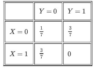
Consider two random variables X and Y with the joint PMF given by the table below.a. Find the linear MMSE estimator of X given Y , (X̂L).b. Find the MMSE estimator of X given Y , (X̂M).c. Find the MSE of X̂ M. X = 0 X = 1 Y = 0 =0 7/12 3 7 Y Y = 1 3|7 0
Suppose that t he random variable X is transmitted over a communication channel. Assume that the received signal is given by Y = X +W, where W ∼ N(0,σ2) is independent of X. Suppose that X = 1 with probability p, and X = −1 with probability 1 −p. The goal is to decide between X = 1 and X =
Find the average error probability in Example 9.10Example 9.10Suppose that t he random variable X is transmitted over a communication channel. Assume that the received signal is given by Y = X +W, where W ∼ N(0,σ2) is independent of X. Suppose that X = 1 with probability p, and X = −1 with
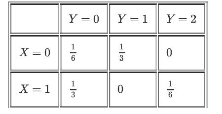
Consider two random variables X and Y with the joint PMF given by the table below.a. Find the linear MMSE estimator of X given Y , ( X̂L).b. Find the MSE of X̂L.c. Find the MMSE estimator of X given Y , ( X̂M).d. Find the MSE of X̂M. Y=0| Y = 1 1 X = 0 증 X = 1 1 3 1 3 0 Y Y=2 0 1 6
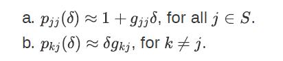
Explain why the following approximations hold: a. pjj (8) b. pkj (6) 1+9jjd, for all j = S. 8gkj, for k ‡ j.
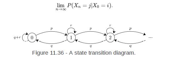
Consider the Markov chain shown in Figure 11.36. Assume that 0 < p < q. Does this chain have a limiting distribution? For all i, j ∈ {0, 1, 2,⋯}, find
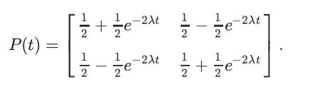
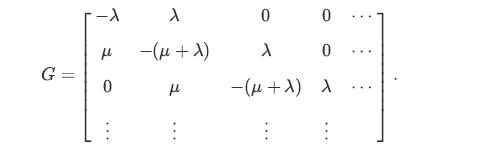
Consider the co ntinuous Markov chain of Example 11.17: A chain with two states S = {0, 1} and λ0 = λ1 = λ > 0. In that example, we found that the transition matrix for any t ≥ 0 is given bya. Find the generator matrix G.b. Show that for any t ≥ 0, we havewhere P ′(t) is the derivative
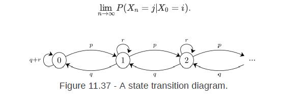
Consider the Markov chain shown in Figure 11.37. Assume that p > q > 0. Does this chain have a limiting distribution? For all i, j ∈ {0, 1, 2,⋯}, find q+r P 9 lim P(Xn=jXo = i). n→∞ P 9 P 9 Figure 11.37 - A state transition diagram.
The generator matrix for the continuous Markov chain of Example 11.17 is given byFind the stationary distribution for this chain by solving πG = 0.Example 11.17Consider a continuous Markov chain with two states S = {0, 1}. Assume the holding time parameters are given by λ0 = λ1 = λ > 0. That
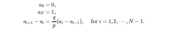
Two gamblers, call them Gambler A and Gambler B, play repeatedly. In each round, A wins 1 dollar with probability p or loses 1 dollar with probability q = 1 −p (thus, equivalently, in each round B wins 1 dollar with probability q = 1 −p and loses 1 dollar with probability p). We assume
Let W(t) be a standard Brownian motion. For all s, t ∈ [0,∞), find CW(s, t) = Cov(W(s),W(t)).
Let N = 4 and i = 2 in the gambler's ruin problem. Find the expected number of rounds the gamblers play until one of them wins the game.
Let W(t) be a standard Brownian motion.a. Find P(1 < W(1) < 2).b. Find P(W(2) < 3|W(1) = 1).
The Poisson process is a continuous-time Markov chain. Specifically, let N(t) be a Poisson process with rate λ.a. Draw the state transition diagram of the corresponding jump chain.b. What are the rates λi for this chain?
Consider a continuous-time Markov chain X(t) that has the jump chain shown in Figure 11.38. Assume λ1 = λ2 = λ3, and λ4 = 2λ1. H 1 4 1 2 3 1 Figure 11.38 - The jump chain for the Markov chain of Problem 26.
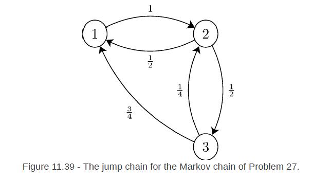
Consider a continuous-time Markov chain X(t) that has the jump chain shown in Figure 11.39. Assume λ1 = 1, λ2 = 2, and λ3 = 4.a. Find the generator matrix for this chain.b. Find the limiting distribution for X(t) by solving πG = 0. 1 تار 1 14 2 3 Figure 11.39 - The jump chain for the Markov
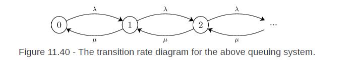
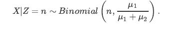
Consider the queuing system of Problem 3 in the Solved Problems Section. Specifically, in that problem we found the following generator matrix and transition rate diagram:The transition rate diagram is shown in Figure 11.40Assume that 0 Problem 3Let X ∼ Poisson(μ1) and Y ∼ Poisson(μ2) be two
Let W(t) be the standard Brownian motion.a. Find P(−1 < W(1) < 1).b. Find P(1 < W(2) +W(3) < 2).c. Find P(W(1) > 2|W(2) = 1).
Let W(t) be a standard Brownian motion. FindP(0 < W(1) +W(2) < 2, 3W(1) −2W(2) > 0).
Let W(t) be a standard Brownian motion. DefineNote that X(0) = X(1) = 0. Find Cov(X(s),X(t)), for 0 ≤ s ≤ t ≤ 1. X(t) = W(t) - tW (1), for all t € [0,00).
Let W(t) be a standard Brownian motion. Let a > 0. Define Ta as the first time that W(t) = a. That isa. Show that for any t ≥ 0, we haveb. Using Part (a), show thatc. Using Part (b), show that the PDF of Ta is given byBy symmetry of Brownian motion, we conclude that for any a ≠ 0, we have Ta
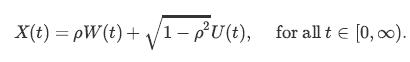
Let W(t) and U(t) be two independent standard Brownian motions. Let −1 ≤ ρ ≤ 1. Define the random process X(t) asa. Show that X(t) is a standard Brownian motion.b. Find the covariance and correlation coefficient of X(t) and W(t). That is, find Cov(X(t),W(t)) and ρ(X(t),W(t)). X(t) = pW (t)
Simulate tossing a coin with probability of heads p.
Write codes to simulate tossing a fair coin to see how the law of large numbers works.
Generate a Binomial(50; 0:2) random variable.
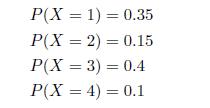
Give an algorithm to simulate the value of a random variable X such that P(X= 1) = 0.35 P(X2) = 0.15 P(X= 3) = 0.4 P(X= 4) = 0.1
Generate an Exponential(1) random variable.
Generate a Gamma(20,1) random variable.
Generate a Poisson random variable. In this example, use the fact that the number of events in the interval [0; t] has Poisson distribution when the elapsed times between the events are Exponential.
Generate 5000 pairs of normal random variables and plot both histograms.
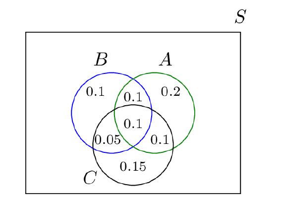
Let A,B, and C be three events with probabilities given below:a. Find P(A|B).b. Find P(C|B).c. Find P(B|A ∪ C).d. Find P(B|A,C) = P(B|A ∩ C). В 0.1 (0.05 C 0.1 0.1 0.15 A 0.2 0.1 S
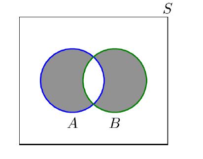
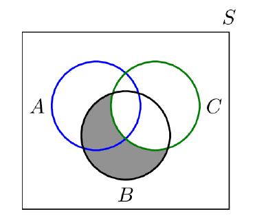
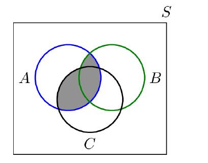
For each of the following Venn diagrams, write the set denoted by the shaded area.a.b.c.d. A B S
Suppose th at the universal set S is defined as S = {1, 2,⋯, 10} and A = {1, 2, 3}, B = {X ∈ S : 2 ≤ X ≤ 7}, and C = {7, 8, 9, 10}.a. Find A ∪ B.b. Find (A ∪ C) −B.c. Find Ā ∪ (B −C).d. Do A,B, and C form a partition of S?
The following sets are used in this book:The set of natural numbers, N = {1, 2, 3,⋯}.The set of integers, Z = {⋯,−3,−2,−1, 0, 1, 2, 3,⋯}.The set of rational numbers Q.The set of real numbers R.Closed intervals on the real line. For example, [2, 3] is the set of all real numbers x such
When working with real numbers, our universal set is R. Find each of the following sets.a. [6, 8] ∪ [2, 7)b. [6, 8] ∩ [2, 7)c. [0, 1]cd. [6, 8]−(2, 7)
Here are som e examples of sets defined by stating the properties satisfied by the elements:If the set C is defined as C = {x|x ∈ Z,−2 ≤ x < 10}, then C = {−2,−1, 0,⋯, 9}.If the set D is defined as D = {x2|x ∈ N}, then D = {1, 4, 9, 16,⋯}.The set of rational numbers can be defined
Here are some examples of sets and their subsets:If E = {1, 4} and C = {1, 4, 9}, then E ⊂ C.N ⊂ Z.Q ⊂ R.
A coin is tossed twice. Let S be the set of all possible pairs that can be observed, i.e., S = {H,T} ×{H,T} = {(H,H), (H,T), (T,H), (T,T)}. Write the following sets by listing their elements.a. A: The first coin toss results in head.b. B: At least one tail is observed.c. C: The two coin tosses
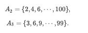
Let A = {1, 2,⋯, 100}. For any i ∈ N, Define Ai as the set of numbers in A that are divisible by i. For example:a. Find |A2|,|A3|,|A4|,|A5|.b. Find |A2 ∪ A3 ∪ A5|. A₂ = {2,4,6,, 100}, As {3,6,9,,99}.
If the universa l set is given by S = {1, 2, 3, 4, 5, 6}, and A = {1, 2}, B = {2, 4, 5},C = {1, 5, 6} are three sets, find the following sets:a. A ∪ Bb. A ∩ Bc. Ād. B̄e. Check De Morgan's law by finding (A ∪ B)c and Ac ∩ Bc.f. Check the distributive law by finding A ∩ (B ∪ C) and (A
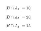
Suppose th at A1, A2, A3 form a partition of the universal set S. Let B be an arbitrary set. Assume that we knowFind |B|. BnA₁ BnA₂ BnA₂ = 10, = 20, = 15.
In a party,There are 10 people with white shirts and 8 people with red shirts;4 people have black shoes and white shirts;3 people have black shoes and red shirts; The total number of people with white or red shirts or black shoes is 21.How many people have black shoes?
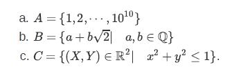
Determine whether each of the following sets is countable or uncountable. a. A = {1,2,, 10¹0} b. B = {a+b√2 a, b = Q} C. C = {(X,Y) = R²| x² + y² ≤ 1}.
Showing 6800 - 6900
of 7136
First
58
59
60
61
62
63
64
65
66
67
68
69
70
71
72
Step by Step Answers


![XL = CXYCY (Y - E[Y]) + E[X].](https://dsd5zvtm8ll6.cloudfront.net/images/question_images/1698/3/8/2/586653b42fa5dcc41698382585572.jpg)
![A]. [xx] = 0 Y- G](https://dsd5zvtm8ll6.cloudfront.net/images/question_images/1698/3/8/9/455653b5dcf972781698389453241.jpg)
![2 i-17 9 = [ + + ( ) + + + ( ) ^ ] - 9 P P P a, for i=1,2,..., N.](https://dsd5zvtm8ll6.cloudfront.net/images/question_images/1698/3/9/3/888653b6f209d9e31698393883997.jpg)
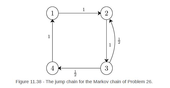
![a. Find the stationary distribution of the jump chain = [1,2,3,4]. b. Using , find the stationary](https://dsd5zvtm8ll6.cloudfront.net/images/question_images/1698/3/9/3/968653b6f700940f1698393962897.jpg)
![P(Ta t)=21-0 a (+7)] t](https://dsd5zvtm8ll6.cloudfront.net/images/question_images/1698/3/9/4/413653b712dbd55b1698394413371.jpg)