New Semester Started Get 50% OFF Study Help! --h --m --s Claim Now

Question Answers

Textbooks

Find textbooks, questions and answers

Oops, something went wrong!

Change your search query and then try again

Result Not Found

Books FREE
Study Help
Tutors
AI Study Planner NEW
Sell Books

Search
Sign In
Register

study help
business
introduction to probability statistics

Probability And Statistics For Engineers 9th Global Edition Richard Johnson, Irwin Miller, John Freund - Solutions

Show that if \(\mu_{i j}=\mu+\alpha_{i}+\beta_{j}\), the mean of the \(\mu_{i j}\) (summed on \(j\) ) is equal to \(\mu+\alpha_{i}\), and the mean of \(\mu_{i j}\) (summed on \(i\) and \(j\) ) is equal to \(\mu\), it follows that\[\sum_{i=1}^{a} \alpha_{i}=\sum_{j=1}^{b} \beta_{j}=0\]
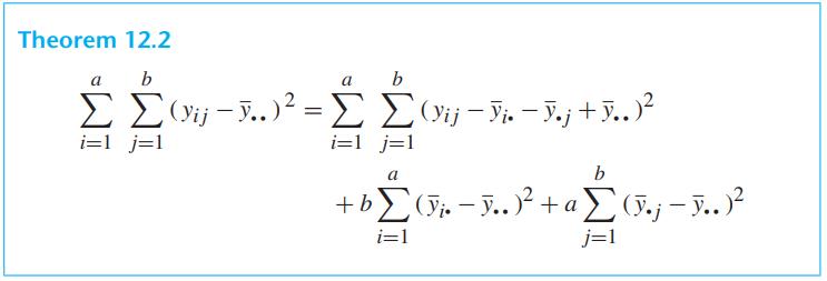
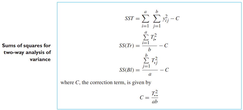
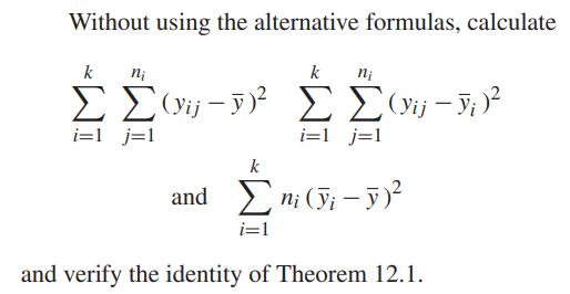
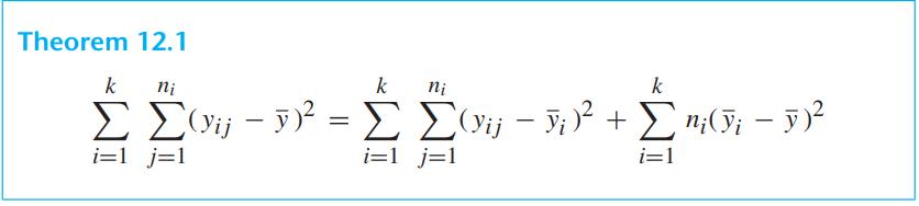
Verify that the computing formulas for \(S S T, S S(T r)\), \(S S(B l)\), and \(S S E\), given on page 409 , are equivalent to the corresponding terms of the identity of Theorem 12.2.Data From Theorem 12.2Data From Page 409 Theorem 12.2 a b a b (ij..)= (Vij Fix Yoj + Y.. ) i=1 j=1 i=1 j=1 b
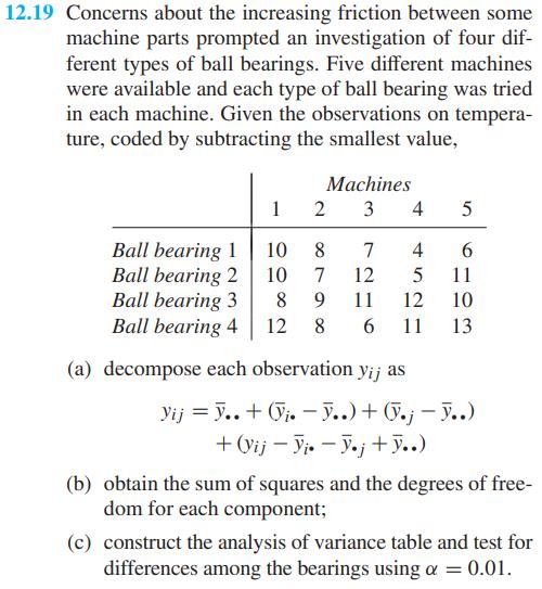
Using \(q_{0.01}=5.499\) for the Tukey HSD method, examine differences among the ball bearings in Exercise 12.19.Data From Exercise 12.19 12.19 Concerns about the increasing friction between some machine parts prompted an investigation of four dif- ferent types of ball bearings. Five different
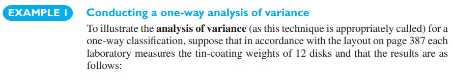
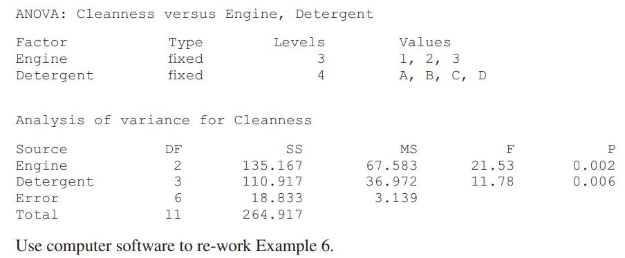
Referring to Example 1, use \(q_{0.05}=3.776\) for the Tukey HSD method to examine differences in mean coating weights.Data From Example 1 EXAMPLE I Conducting a one-way analysis of variance To illustrate the analysis of variance (as this technique is appropriately called) for a one-way
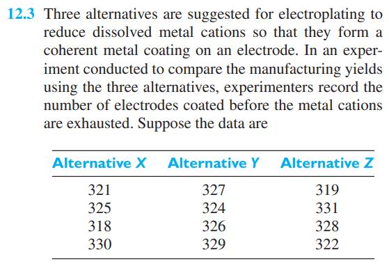
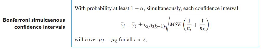
Referring to Exercise 12.3, use Bonferroni simultaneous confidence intervals with \(\alpha=0.06\) to compare the mean number of electrodes coated by the experiment under the 3 different alternatives.Data From Exercise 12.3Data From Theorem 12.1 12.3 Three alternatives are suggested for
An approximation to Tukey HSD confidence intervals for mildly unequal sample sizes When the there are only small differences in the sample sizes, an approximation is available. The MSE and its degrees of freedom still come from the ANOVA table but \(\sqrt{2 M S E / n}\) is replaced by\[\sqrt{M S
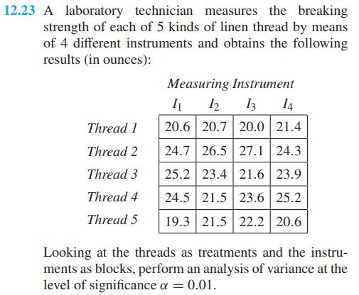
(a) Using \(q_{0.10}=3.921\) for the Tukey HSD method, compare the strength of the 5 linen threads in Exercise 12.23 .(b) Use the Bonferroni confidence interval approach on page 411, with \(\alpha=0.10\), to compare the mean linen thread strengths in Exercise 12.20.Data From Exercise 12.23Data From
The Bonferroni inequality states that\[P\left(\cap_{i} C_{i}\right) \geq 1-\sum_{i} P\left(\overline{C_{i}}\right)\](a) Show that this holds for 3 events.(b) Let \(C_{i}\) be the event that the \(i\) th confidence interval will cover the true value of the parameter for \(i=1, \ldots, m\). If
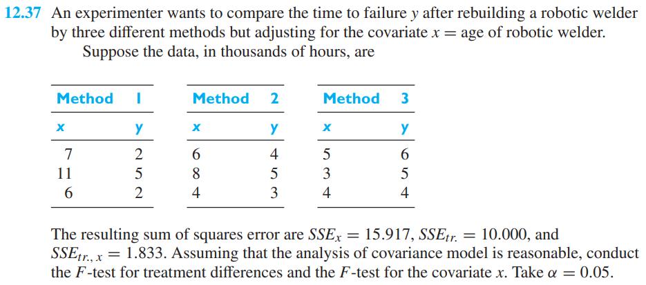
An experimenter wants to compare the time to failure \(y\) after rebuilding a robotic welder by three different methods but adjusting for the covariate \(x=\) age of robotic welder.Suppose the data, in thousands of hours, areThe resulting sum of squares error are \(S S E_{x}=15.917, S S E_{t
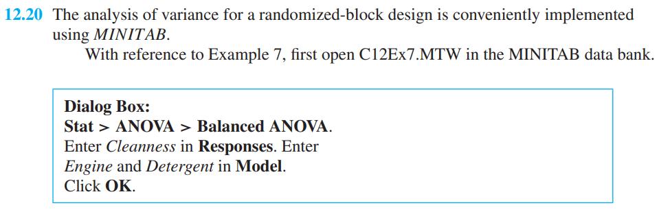
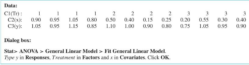
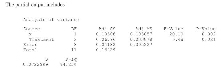
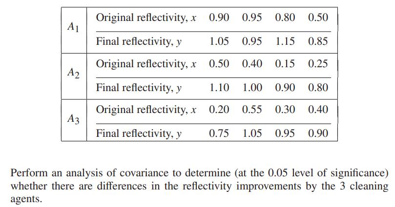
MINITAB calculation of balanced analysis of covariance We illustrate the MINTAB commands for Example 11 concerning surface reflectivity.Use computer software to perform an analysis of covariance for the fitness wristband.Data From Example 11 Data: C1(Tr): 1 1 1 1 2 2 2 2 3 3 3 3 C2(x): 0.90 0.95
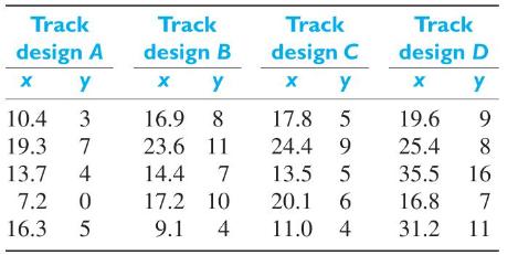
Four different railroad-track cross-section configurations were tested to determine which is most resistant to breakage under use conditions. Ten miles of each kind of track were laid in each of 5 locations, and the number of cracks and other fracture-related conditions (y) was measured over a
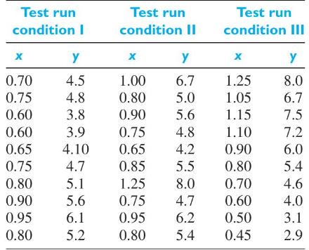
To compare power consumption by a newly developed low-power USB device under three test run conditions and record the data transmission rate at the same time, a computer engineer obtained the following results, where the power consumption, \(x\), is in Watts, and the data transmission rate, \(y\),
Use computer software to work Exercise 12.37.Data From Exercise 12.37 12.37 An experimenter wants to compare the time to failure y after rebuilding a robotic welder by three different methods but adjusting for the covariate x = age of robotic welder. Suppose the data, in thousands of hours, are x
Assume the following data obey the one-way analysis of variance model.(a) Decompose each observation \(y_{i j}\) as \[y_{i j}=\bar{y}+\left(\bar{y}_{i}-\bar{y}\right)+\left(y_{i j}-\bar{y}_{i}\right)\](b) Obtain the sums of squares and degrees of freedom for each array.(c) Construct the analysis of
To determine the effect of height on power generated in a hydroelectric power plant, the following observations were made:.Use the level of significance \(\alpha=0.05\) to test whether the height of the reservoir has an effect on the power generated. Total height (m) Power generated (megawatts per
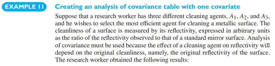
Refer to Example 11. Ignore the covariate original reflectivity. Perform an analysis of variance take \(\alpha=0.05\)Data From Example 11 EXAMPLE II Creating an analysis of covariance table with one covariate Suppose that a research worker has three different cleaning agents, A1, A2, and A3, and he
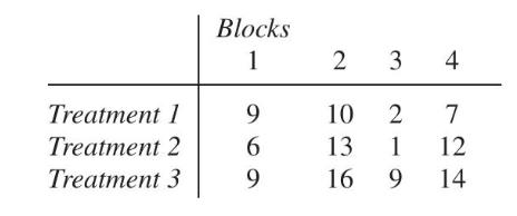
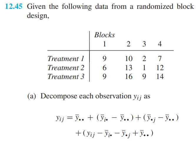
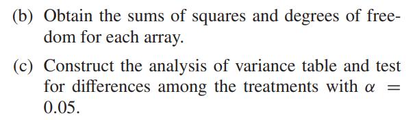
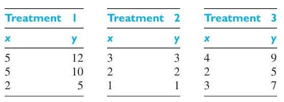
Given the following data from a randomized block design,(a) Decompose each observation \(y_{i j}\) as \[\begin{aligned} y_{i j}= & \bar{y}_{\bullet}+\left(\bar{y}_{\bullet \bullet}-\bar{y}_{\bullet \bullet}\right)+\left(\bar{y}_{\bullet j}-\bar{y}_{\bullet \bullet}\right) \\ & +\left(y_{i
Using \(q_{0.05}=4.339\) for the Tukey HSD method, compare the treatments in Exercise 12.45.Data From Exercise 12.45 12.45 Given the following data from a randomized block design, Blocks 1 234 Treatment 1 9 10 2 7 Treatment 2 6 13 1 12 Treatment 3 9 16 9 14 (a) Decompose each observation yij as Yij
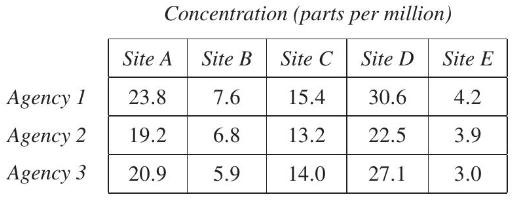
Samples of groundwater were taken from 5 different toxic-waste dump sites by each of 3 different agencies: the EPA, the company that owned each site, and an independent consulting engineer. Each sample was analyzed for the presence of a certain contaminant by whatever laboratory method was
Using \(q_{0.05}=4.041\) for the Tukey HSD method, compare the pollution levels of the three agencies in Exercise 12.47.Data From Exercise 12.47 12.47 Samples of groundwater were taken from 5 different toxic-waste dump sites by each of 3 different agen- cies: the EPA, the company that owned each
An experiment is conducted with \(k=5\) treatments, one covariate \(x\), and \(n=6\). Calculations result in the sums of squares error \(S S E_{x}=14.4, S S E_{t r}=4.69\), and \(S S E_{t r, x}=1.21\). Assuming that the analysis of covariance model is reasonable, conduct the \(F\)-test for
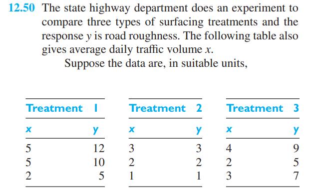
The state highway department does an experiment to compare three types of surfacing treatments and the response \(y\) is road roughness. The following table also gives average daily traffic volume \(x\).Suppose the data are, in suitable units,(a) Perform an analysis of variance on the response
Refer to Exercise 12.50.(a) Perform an analysis of covariance. Test for a difference in treatments using level of significance 0.05 .(b) Compare your analysis in part (a) with the analysis of variance. Is the covariate important?Data From Exercise 12.50 12.50 The state highway department does an
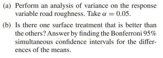
Three different instrument panel configurations were tested by placing airline pilots in flight simulators and testing their reaction time to simulated flight emergencies. Eight pilots were assigned to each instrument panel configuration. Each pilot was faced with 10 emergency conditions in a
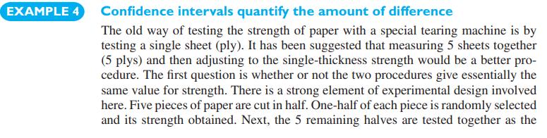
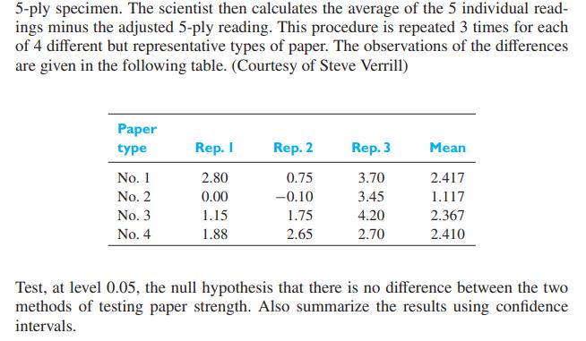
Using the alternative calculation formula verify analysis of variance table for the paper-strength in Example 4.Data From Example 4 EXAMPLE 4 Confidence intervals quantify the amount of difference The old way of testing the strength of paper with a special tearing machine is by testing a single
Benjamin Franklin (1706-1790) conducted an experiment to study the effect of water depth on the amount of drag on a boat being pulled up a canal. He made a 14-foot trough and a model boat 6 inches long. A thread was attached to the bow, put through a pulley, and then a weight was attached. Not
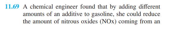
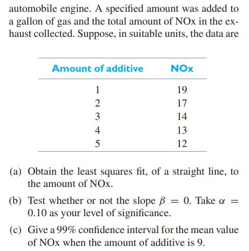
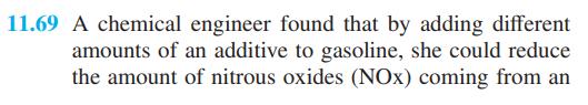
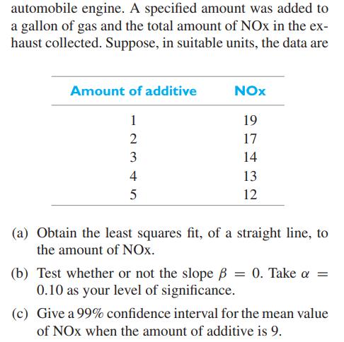
A chemical engineer found that by adding different amounts of an additive to gasoline, she could reduce the amount of nitrous oxides (NOx) coming from an automobile engine. A specified amount will be added to a gallon of gas and the total amount of NOx in the exhaust collected. Initially, five runs
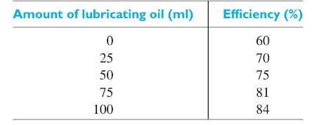
A motorist found that the efficiency of her engine could be increased by adding lubricating oil to fuel. She experimented with different amounts of lubricating oil and the data are(a) Obtain the least squares fit of a straight line to the amount of lubricating oil.(b) Test whether or not the slope
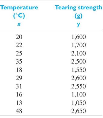
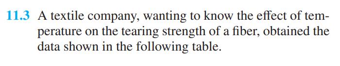
A textile company, wanting to know the effect of temperature on the tearing strength of a fiber, obtained the data shown in the following table.(a) Draw a scatter plot to verify that a straight line will provide a good fit to the data, draw a straight line by eye, and use it to predict the tearing
In the accompanying table, \(x\) is the tensile force applied to a steel specimen in thousands of pounds, and \(y\) is the resulting elongation in thousandths of an inch:(a) Graph the data to verify that it is reasonable to assume that the regression of \(Y\) on \(x\) is linear.(b) Find the
With reference to the preceding exercise,(a) construct a \(95 \%\) confidence interval for \(\beta\), the elongation per thousand pounds of tensile stress;(b) find 95% limits of prediction for the elongation of a specimen with \(x=3.5\) thousand pounds.
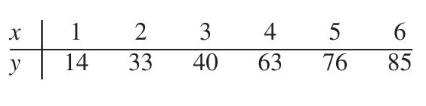
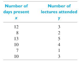
The following table shows how many days in December a sample of 6 students were present at their university and the number of lectures each attended on a given day.(a) Find the equation of the least squares line which will enable us to predict \(y\) in terms of \(x\).(b) Use the result in part (a)
With reference to the preceding exercise, test the null hypothesis \(\beta=0.75\) against the alternative hypothesis \(\beta
With reference to Exercise 11.6, find(a) a \(90\%\) confidence interval for the average number of classes attended each day by a student present for 15 days;(b) \(90 \%\) limits of prediction for the number of classes attended each day by a student present for 15 days.Data From Exercise 11.6 11.6
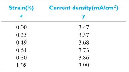
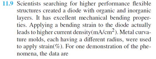
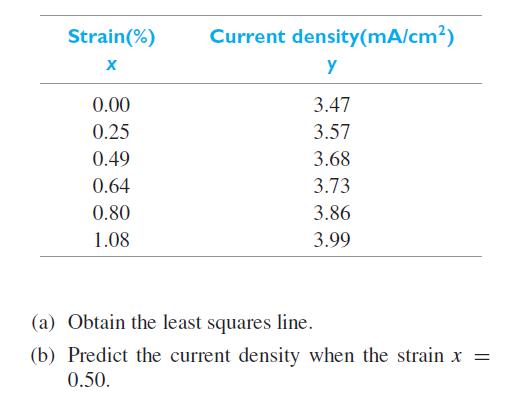
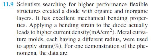
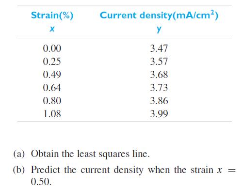
Scientists searching for higher performance flexible structures created a diode with organic and inorganic layers. It has excellent mechanical bending properties. Applying a bending strain to the diode actually leads to higher current density \(\left(\mathrm{mA} / \mathrm{cm}^{2}\right)\). Metal
With reference to Exercise 11.9, construct a 95% confidence interval for \(\alpha\).Data From Exercise 11.9 11.9 Scientists searching for higher performance flexible structures created a diode with organic and inorganic layers. It has excellent mechanical bending proper- ties. Applying a bending
With reference to Exercise 11.9, test the null hypothesis \(\beta=0.40\) against the alternative hypothesis \(\beta>\) 0.40 at the 0.05 level of significance.Data From Exercise 11.9 11.9 Scientists searching for higher performance flexible structures created a diode with organic and inorganic
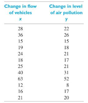
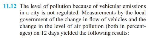
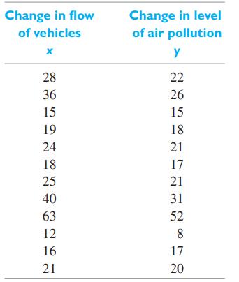
The level of pollution because of vehicular emissions in a city is not regulated. Measurements by the local government of the change in flow of vehicles and the change in the level of air pollution (both in percentages) on 12 days yielded the following results:(a) Make a scatter plot to verify that
With reference to the preceding exercise, find \(99 \%\) limits of prediction for the level of air pollution when the flow of vehicles is \(30 \%\). Also indicate to what extent the width of the interval is affected by the size of the sample and to what extent it is affected by the inherent
With reference to Exercise 11.3, express \(90 \%\) limits of prediction for the tearing strength in terms of the temperature \(x_{0}\). Choosing suitable values of \(x_{0}\), sketch graphs of the loci of upper and lower limits of prediction on the diagram of part (a) of Exercise 11.3. Note that
In Exercise 11.4 it would have been entirely reasonable to impose the condition \(\alpha=0\) before fitting a straight line by the method of least squares.(a) Use the method of least squares to derive a formula for estimating \(\beta\) when the regression line has the form \(y=\beta x\).(b) With
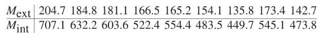
Recycling concrete aggregate is an important component of green engineering. The strength of any potential material, expressed in terms of its resilient modulus, must meet standards before it is incorporated in the base of new roadways. There are two methods of obtaining the resilient modulus. The
With reference to Exercise 11.16, find a \(90 \%\) confidence interval for \(\alpha\).Data From Exercise 11.16 11.16 Recycling concrete aggregate is an important compo- nent of green engineering. The strength of any po- tential material, expressed in terms of its resilient modulus, must meet
With reference to Exercise 11.16, fit a straight line to the data by the method of least squares, using \(M_{\text {ext }}\) as the independent variable, and draw its graph on the diagram obtained in part (a) of Exercise 11.16. Note that the two estimated regression lines do not coincide.Data From
When the sum of the \(x\) values is equal to zero, the calculation of the coefficients of the regression line of \(Y\) on \(x\) is greatly simplified; in fact, their estimates are given by\[\widehat{\alpha}=\frac{\sum y}{n} \text { and } \quad \widehat{\beta}=\frac{\sum x y}{\sum x^{2}}\]This
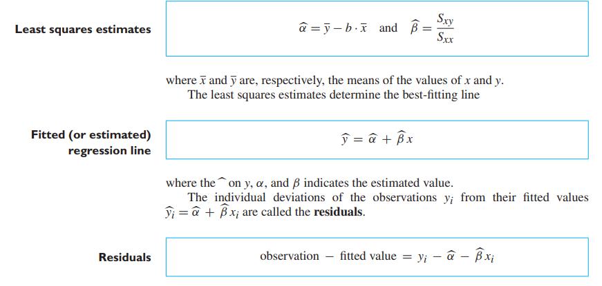
Using the formulas on page 330 for \(\widehat{\alpha}\) and \(\widehat{\beta}\), show that(a) the expression for \(\widehat{\alpha}\) is linear in the \(Y_{i}\)(b) \(\widehat{\alpha}\) is an unbiased estimate of \(\alpha\)(c) the expression for \(\widehat{\beta}\) is linear in the \(Y_{i}\)(d)
The decomposition of the sums of squares into a contribution due to error and a contribution due to regression underlies the least squares analysis. Consider the identity\[y_{i}-\bar{y}-\left(\widehat{y}_{i}-\bar{y}\right)=\left(y_{i}-\widehat{y}_{i}\right)\]Note that\[\begin{aligned} &
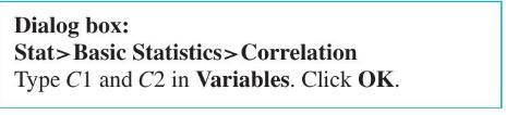
It is tedious to perform a least squares analysis without using a computer. We illustrate here a computer-based analysis using the MINITAB package. The observations on page 328 are entered in \(\mathrm{C} 1\) and \(\mathrm{C} 2\) of the worksheet.We first obtain the scatter plot to see if a
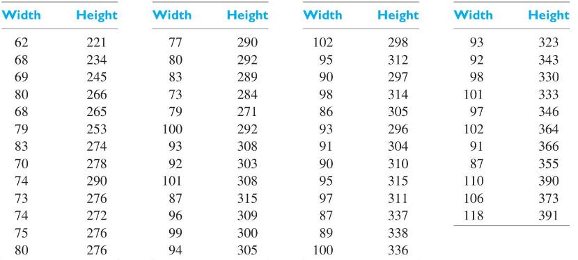
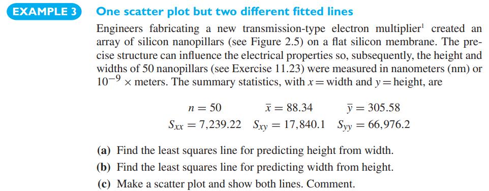
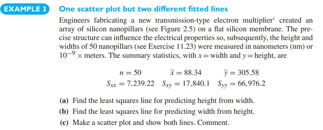
Referring to Example 3, the nanopillar data on height (nm) and width ( \(\mathrm{nm})\) are(a) Fit a straight line with \(y=\) height and \(x=\) width by least squares.(b) Test, with \(\alpha=0.05\), that the slope is different from zero.(c) Find a 95% confidence interval for the mean height when
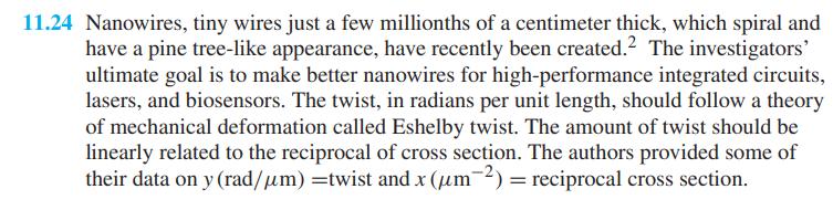
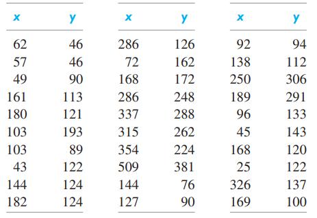
Nanowires, tiny wires just a few millionths of a centimeter thick, which spiral and have a pine tree-like appearance, have recently been created. \({ }^{2}\) The investigators' ultimate goal is to make better nanowires for high-performance integrated circuits, lasers, and biosensors. The twist, in
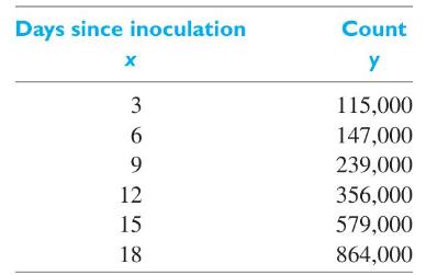
The following data pertain to the growth of a colony of bacteria in a culture medium:(a) Plot \(\log y_{i}\) versus \(x_{i}\) to verify that it is reasonable to fit an exponential curve.(b) Fit an exponential curve to the given data.(c) Use the result obtained in part (b) to estimate the bacteria
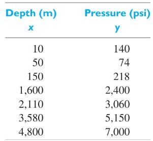
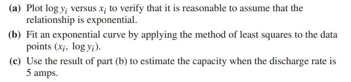
The following data pertain to water pressure at various depths below sea level:(a) Fit an exponential curve.(b) Use the result obtained in part (a) to estimate the mean pressure at a depth of \(1,000 \mathrm{~m}\). Depth (m) Pressure (psi) x y 10 140 50 74 150 218 1,600 2,400 2,110 3,060 3,580
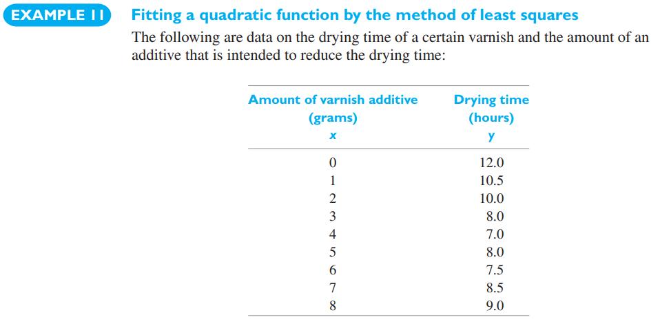
With reference to the preceding exercise, change the equation obtained in part (a) to the form \(\widehat{y}=a \cdot e^{-c x}\), and use the result to rework part (b).
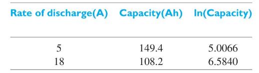
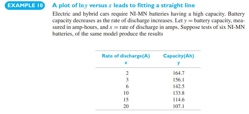
Refer to Example 10. Two new observations are available.Add these observations to the data set in Example 10 and rework the example.Data From Example 10 Rate of discharge (A) Capacity (Ah) In(Capacity) 5 149.4 5.0066 18 108.2 6.5840
Fit a Gompertz curve of the form \[y=e^{e^{\alpha x+\beta}}\] to the data of Exercise 11.26.Data From Exercise 11.26 11.26 The following data pertain to water pressure at various depths below sea level: Depth (m) Pressure (psi) x y 10 140 50 74 150 218 1,600 2,400 2,110 3,060 3,580 5,150 4,800
Plot the curve obtained in the preceding exercise and the one obtained in Exercise 11.26 on one diagram and compare the fit of these two curves.Data From Exercise 11.26 11.26 The following data pertain to water pressure at various depths below sea level: Depth (m) Pressure (psi) x y 10 140 50 74
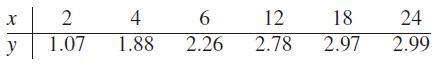
The number of inches which a newly built structure is settling into the ground is given by\[y=3-3 e^{-\alpha x}\]where \(x\) is its age in months.Use the method of least squares to estimate \(\alpha\). That the relationship between \(\ln (3-y)\) and \(x\) is linear.] X 2 4 6 12 18 24 y 1.07 1.88
The following data pertain to the amount of hydrogen present, \(y\), in parts per million in core drillings made at 1 -foot intervals along the length of a vacuum-cast ingot, \(x\), core location in feet from base:(a) Draw a scatter plot to check whether it is reasonable to fit a parabola to the
When fitting a polynomial to a set of paired data, we usually begin by fitting a straight line and using the method on page 339 to test the null hypothesis \(\beta_{1}=0\). Then we fit a second-degree polynomial and test whether it is worthwhile to carry the quadratic term by comparing
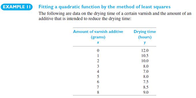
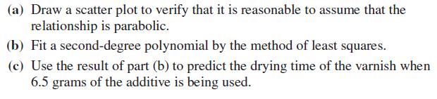
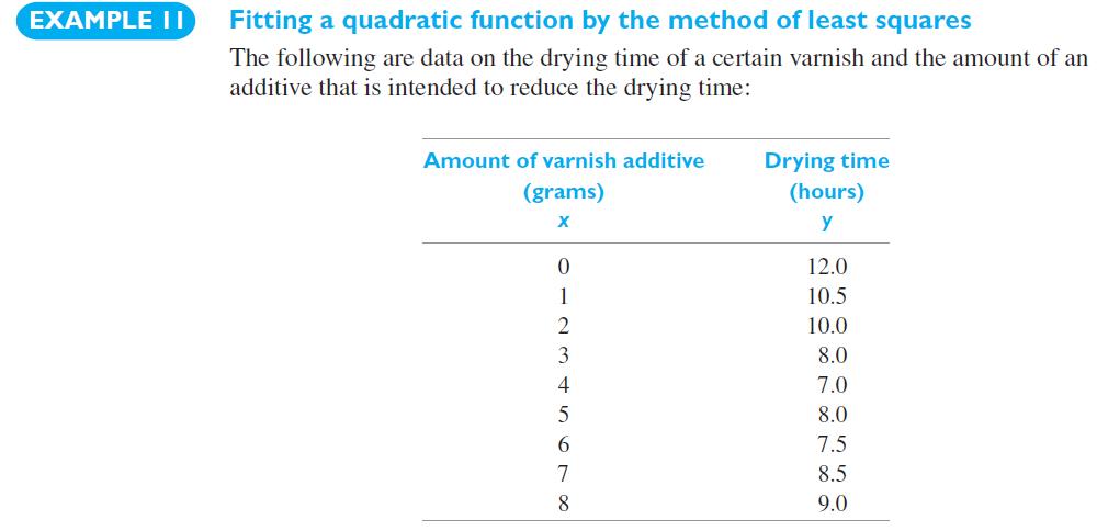
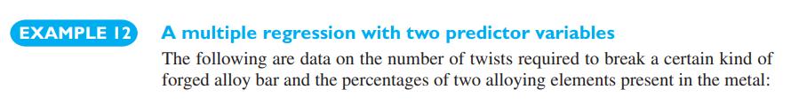
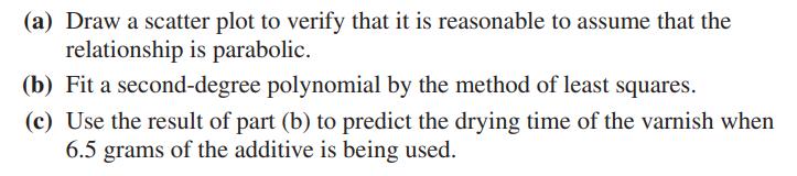
With reference to Example 11, verify that the predicted drying time is minimum when the amount of additive used is 5.1 grams.Data From Example 11 EXAMPLE II Fitting a quadratic function by the method of least squares The following are data on the drying time of a certain varnish and the amount of
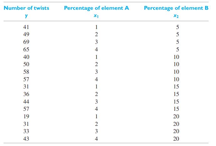
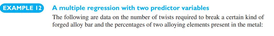
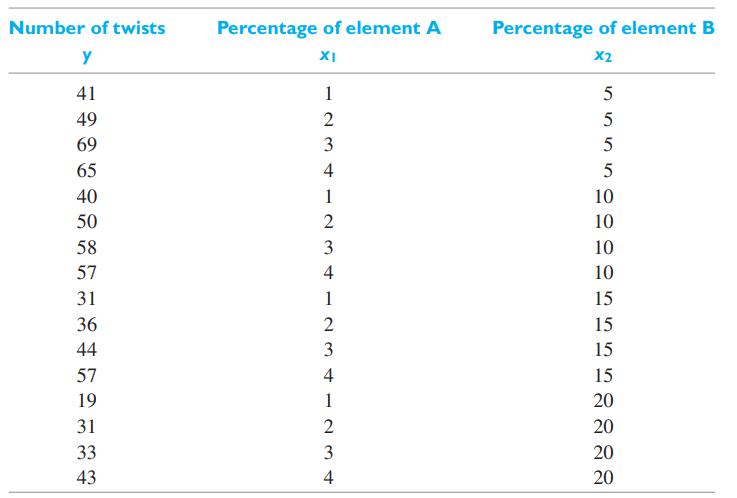
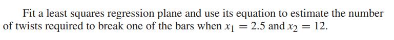
Verify that the system of normal equations on page 357 corresponds to the minimization of the sum of squares. EXAMPLE 12 A multiple regression with two predictor variables The following are data on the number of twists required to break a certain kind of forged alloy bar and the percentages of two
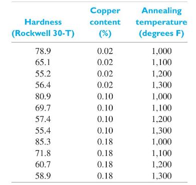
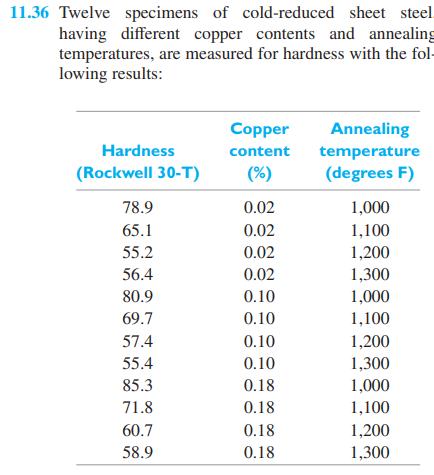
Twelve specimens of cold-reduced sheet steel, having different copper contents and annealing temperatures, are measured for hardness with the following results:Fit an equation of the form \(y=\beta_{0}+\beta_{1} x_{1}+\beta_{2} x_{2}\), where \(x_{1}\) represents the copper content, \(x_{2}\)
With reference to Exercise 11.36, estimate the hardness of a sheet of steel with a copper content of \(0.05 \%\) and an annealing temperature of 1,150 degrees Fahrenheit.Data From Exercise 11.36 11.36 Twelve specimens of cold-reduced sheet steel having different copper contents and annealing
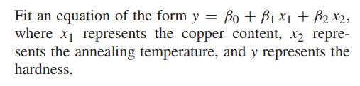
A compound is produced for a coating process. It is added to an otherwise fixed recipe and the coating process is completed. Adhesion is then measured. The following data concern the amount of adhesion and its relation to the amount of an additive and temperature of a reaction.Fit an equation of
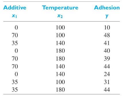
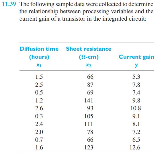
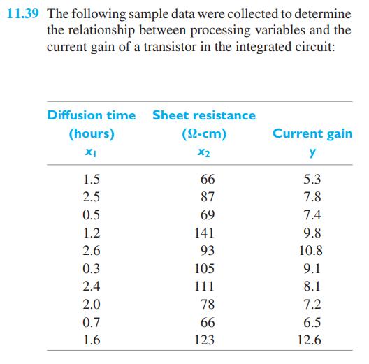
The following sample data were collected to determine the relationship between processing variables and the current gain of a transistor in the integrated circuit:Fit a regression plane and use its equation to estimate the expected current gain when the diffusion time is 2.2 hours and the sheet
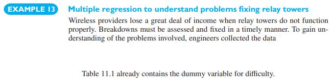
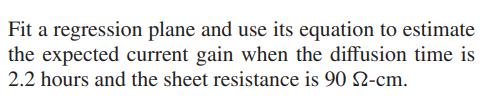
Multiple regression is best implemented on a computer. The following MINITAB commands fits the \(y\) values in \(\mathrm{C} 1\) to predictor values in \(\mathrm{C} 2\) and \(\mathrm{C} 3\).It produces output like that on page 360. Use a computer to perform the multiple regression analysis in
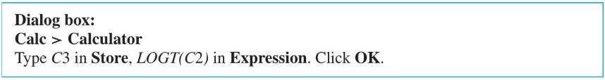
Using MINITAB we can transform the \(x\) values in \(\mathrm{C} 1\) and/or the \(y\) values in \(\mathrm{C} 2\). For instance, to obtain the logarithm to the base 10 of \(y\), selectUse the computer to repeat the analysis of Exercise 11.27.Data From Exercise 11.27 Dialog box: Calc Calculator Type
To fit the quadratic regression model using MINITAB, when the \(x\) values are in C1 and the \(y\) values in \(\mathrm{C} 2\), you must selectUse the computer to repeat the analysis of Example 11.Data From Example 11 Dialog box: Stat Regression > Fitted Line Plot Enter C2 in Response (Y) and enter
With reference to Exercise 11.40, in order to plot residuals, before clicking \(\mathbf{O K}\), you must selectThe additional steps, before clicking the second \(\mathbf{O K}\).will produce a plot of the residuals versus \(\widehat{y}\). See Exercise 5.102, page 184, to obtain a normal-scores plot
With reference to Exercise 11.39, analyze the residuals from the regression plane.Data From Exercise 11.39 11.39 The following sample data were collected to determine the relationship between processing variables and the current gain of a transistor in the integrated circuit: Diffusion time Sheet
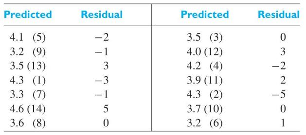
The following residuals and predicted values were obtained from an experiment that related yield of a chemical process \((y)\) to the initial concentration \((x)\) of a component (the time order of the experiments is given in parentheses):Examine the residuals for evidence of a violation of the
Data, collected over seven years, reveals a positive correlation between the annual starting salary of engineers and the annual sales of diet soft drinks. Will buying more diet drinks increase starting salaries? Explain your answer and suggest a possible lurking variable.
Data, collected from cities of widely varying sizes, revealed a high positive correlation between the amount of beer consumed and the number of weddings in the past year. Will consuming lots of beer increase the number of weddings? Explain your answer.
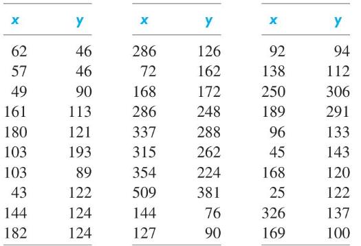
Use the expressions on page 367, involving the deviations from the mean, to calculate \(r\) for the following data: x Y 8278 69 128 10
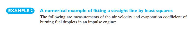
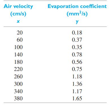
Calculate \(r\) for the air velocities and evaporation coefficients of Example 2. Also, assuming that the necessary assumptions can be met, test the null hypothesis \(ho=0\) against the alternative hypothesis \(ho eq 0\) at the 0.05 level of significance.Data From Example 2 EXAMPLE 2 A numerical
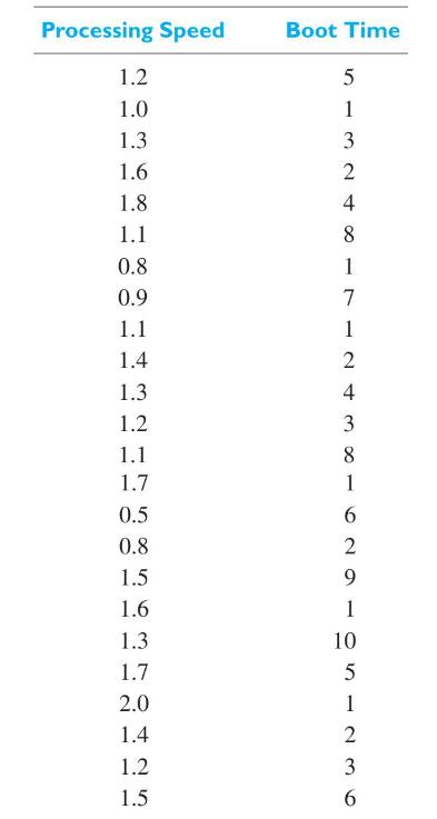
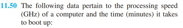
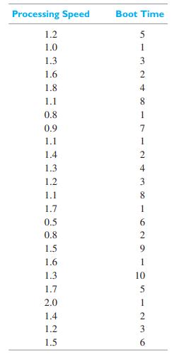
The following data pertain to the processing speed (GHz) of a computer and the time (minutes) it takes to boot up:Calculate \(r\). Processing Speed Boot Time 1.2 5 1.0 1 1.3 1.6 2 1.8 324 3 1.1 8 0.8 1 0.9 7 1.1 1 1.4 2 1.3. 4 1.2 1.1 88 3 1.7 1 0.5 0.8 1.5 629 1.6 1 1.3 10 1.7 2.0 1.4 1.2 1.5 51236
With reference to Exercise 11.50, test \(ho=0\) against \(ho eq 0\) at \(\alpha=0.05\).Data From Exercise 11.50 11.50 The following data pertain to the processing speed (GHz) of a computer and the time (minutes) it takes to boot up:
Calculate \(r\) for the temperatures and tearing strengths of Exercise 11.3. Assuming that the necessary assumptions can be met, test the null hypothesis \(ho=0.60\) against the alternative hypothesis \(ho>0.60\) at the 0.10 level of significance.Data From Exercise 11.3 11.3 A textile company,
Calculate \(r\) for the changes in the flow of vehicles and the level of pollution in Exercise 11.12. Assuming that the necessary assumptions can be met, construct a 99% confidence interval for the population correlation coefficient \(ho\).Data From Exercise 11.12 11.12 The level of pollution
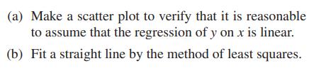
The following are measurements of the total dissolved salts (TDS) and hardness index of 22 samples of water.(a) Calculate \(r\).(b) Find 95% confidence limits for \(ho\). TDS (ppm) Hardness Index 200 15 325 24 110 8 465 34 580 43 925 69 680 50 290 21 775 57 375 28 850 63 625 46 430 32 275 20 170 13
Referring to Example 3 concerning nanopillars, calculate the correlation coefficient between height and width.Data From Example 3 EXAMPLE 3 One scatter plot but two different fitted lines Engineers fabricating a new transmission-type electron multiplier created an array of silicon nanopillars (see
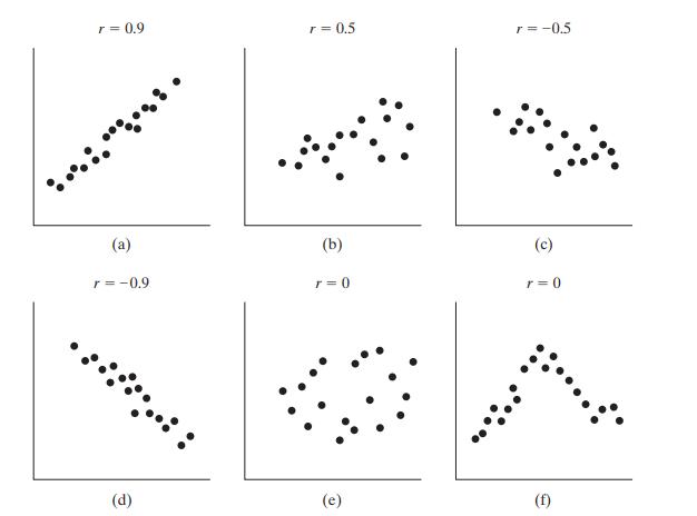
If \(r=0.83\) for one set of paired data and \(r=\) 0.60 for another, compare the strengths of the two relationships.
If data on the ages and prices of 25 pieces of equipment yielded \(r=-0.58\), test the null hypothesis \(ho=-0.40\) against the alternative hypothesis \(ho
Assuming that the necessary assumptions are met, construct a 95% confidence interval for \(ho\) when(a) \(r=0.72\) and \(n=19\);(b) \(r=0.35\) and \(n=25\);(c) \(r=0.57\) and \(n=40\).
(a) Evaluating the necessary integrals, verify the identities\[\mu_{2}=\alpha+\beta \mu_{1} \quad \text { and } \quad \sigma_{2}^{2}=\sigma^{2}+\beta^{2} \sigma_{1}^{2}\]on page 374 .(b) Substitute \(\mu_{2}=\alpha+\beta \mu_{1}\) and \(\sigma_{2}^{2}=\sigma^{2}+\beta^{2} \sigma_{1}^{2}\) into the
Show that for the bivariate normal distribution(a) independence implies zero correlation;(b) zero correlation implies independence.
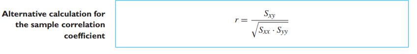
Instead of using the computing formula on page 367, we can obtain the correlation coefficient \(r\) with the formula\[r= \pm \sqrt{1-\frac{\sum(y-\widehat{y})^{2}}{\sum(y-\bar{y})^{2}}}\]which is analogous to the formula used to define \(ho\). Although the computations required by the use of this
With reference to Exercise 11.39, use the theory of the preceding exercise to calculate the multiple correlation coefficient (which measures how strongly the current gain is related to the two independent variables).Data From Exercise 11.39 11.39 The following sample data were collected to
Referring to the nano twisting data in Exercise 11.24, calculate the correlation coefficient.Data From Exercise 11.24 11.24 Nanowires, tiny wires just a few millionths of a centimeter thick, which spiral and have a pine tree-like appearance, have recently been created.2 The investigators' ultimate
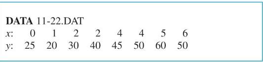
To calculate \(r\) using MINITAB when the \(x\) values are in \(C 1\) and the \(y\) values are in \(C 2\), useAlso, you can make a scatter plot using the plot procedure in Exercise 11.22.Use the computer to do Exercise 11.50.Data From Exercise 11.22Data From Exercise 11.50 Dialog box: Stat>Basic
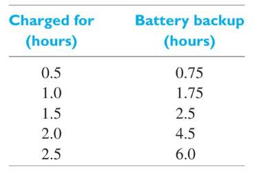
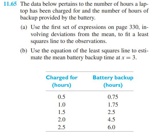
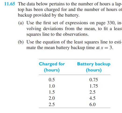
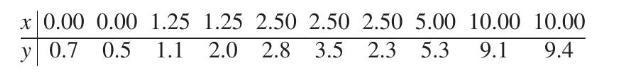
The data below pertains to the number of hours a laptop has been charged for and the number of hours of backup provided by the battery.(a) Use the first set of expressions on page 330, involving deviations from the mean, to fit a least squares line to the observations.(b) Use the equation of the
With reference to Exercise 11.65, construct a \(99 \%\) confidence interval for \(\alpha\).
With reference to Exercise 11.65, test the null hypothesis \(\beta=1.5\) against the alternative hypothesis \(\beta>1.5\) at the 0.01 level of significance.Data From Exercise 11.65 11.65 The data below pertains to the number of hours a lap- top has been charged for and the number of hours of
With reference to Exercise 11.65,(a) find a \(99 \%\) confidence interval for the mean battery backup at \(x=1.25\);(b) find \(95 \%\) limits of prediction for the battery backup provided by a laptop charged for 1.25 hours.Data From Exercise 11.65 11.65 The data below pertains to the number of
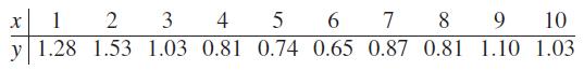
A chemical engineer found that by adding different amounts of an additive to gasoline, she could reduce the amount of nitrous oxides (NOx) coming from an automobile engine. A specified amount was added to a gallon of gas and the total amount of NOx in the exhaust collected. Suppose, in suitable
With reference to Exercise 11.69, find the 95% limits of prediction when the amount of additive is 4.5.Data From Exercise 11.69 11.69 A chemical engineer found that by adding different amounts of an additive to gasoline, she could reduce the amount of nitrous oxides (NOx) coming from an
With reference to Exercise 11.69, find the proportion of variance in the amount of NOx explained by the amount of additive.Data From Exercise 11.69 11.69 A chemical engineer found that by adding different amounts of an additive to gasoline, she could reduce the amount of nitrous oxides (NOx) coming
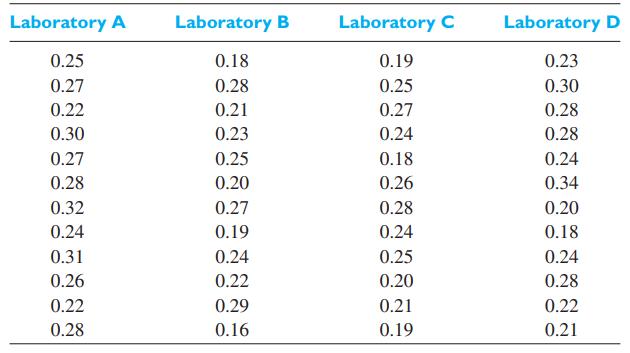
To determine how well existing chemical analyses can detect lead in test specimens in water, a civil engineer submits specimens spiked with known concentrations of lead to a laboratory. The chemists are told only that all samples are from a study about measurements on "low" concentrations, but they
With reference to the preceding exercise, construct a 95% confidence interval for \(\alpha\).
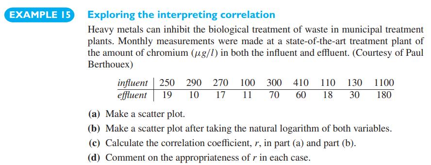
With reference to Example 15,(a) find the least squares line for predicting the chromium in the effluent from that in the influent after taking natural logarithms of each variable;(b) predict the mean \(\ln\) (effluent) when the influent has \(500 \mu \mathrm{g} / \mathrm{l}\) chromium.Data From

Showing 5800 - 5900 of 7136

First
52
53
54
55
56
57
58
59
60
61
62
63
64
65
66
Last

Step by Step Answers

Services

Sitemap
Fun
Definitions
Become Tutor
Used Textbooks
Study Help Categories
Recent Questions
Expert Questions
Campus Wear
Sell Your Books

Company Info

Security
Copyrights
Privacy Policy
Terms & Conditions
SolutionInn Fee
Scholarship
Online Quiz
Give Feedback, Get Rewards

Get In Touch

About Us
Contact Us
Career
Jobs
FAQ
Student Discount
Campus Ambassador

Secure Payment

Download Our App

© 2026 SolutionInn. All Rights Reserved