New Semester Started Get 50% OFF Study Help! --h --m --s Claim Now

Question Answers

Textbooks

Find textbooks, questions and answers

Oops, something went wrong!

Change your search query and then try again

Result Not Found

Books FREE
Study Help
Tutors
AI Study Planner NEW
Sell Books

Search
Sign In
Register

study help
business
introduction to probability statistics

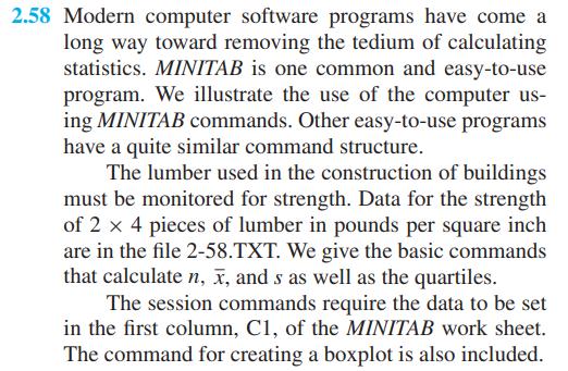
Probability And Statistics For Engineers 9th Global Edition Richard Johnson, Irwin Miller, John Freund - Solutions

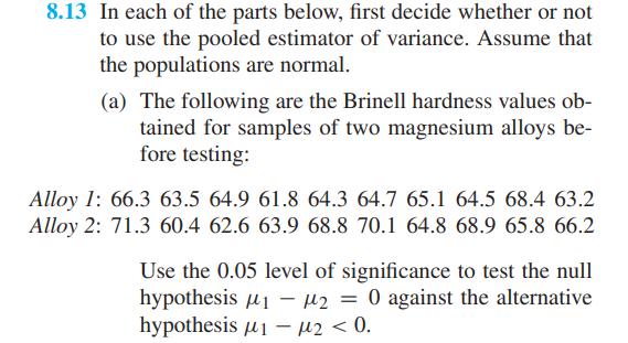
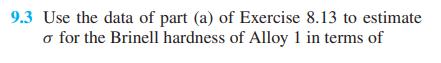
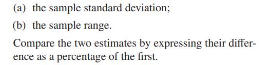
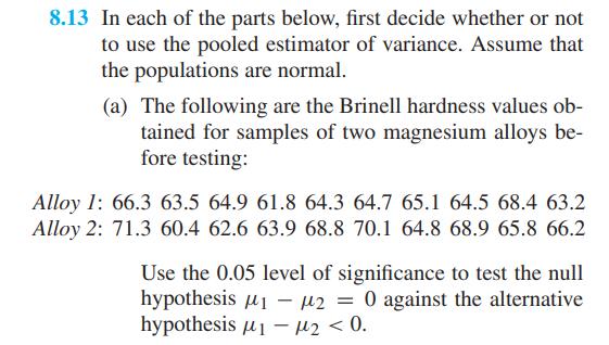
Use the data of part(a) of Exercise 8.13 to estimate \(\sigma\) for the Brinell hardness of Alloy 1 in terms of (a) the sample standard deviation;(b) the sample range.Compare the two estimates by expressing their difference as a percentage of the first.Data From Exercise 8.13 8.13 In each of the
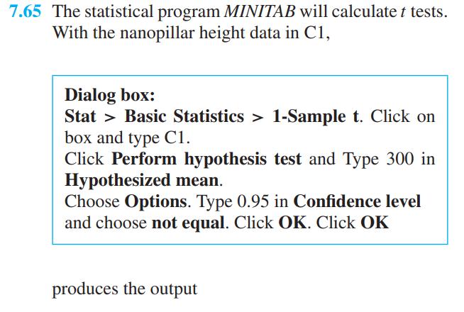
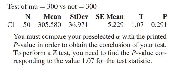
With reference to Exercise 7.56, construct a 95% confidence interval for the variance of the yield.Data From Exercise 7.56 7.65 The statistical program MINITAB will calculate t tests. With the nanopillar height data in C1, Dialog box: Stat Basic Statistics > 1-Sample t. Click on box and type C1.
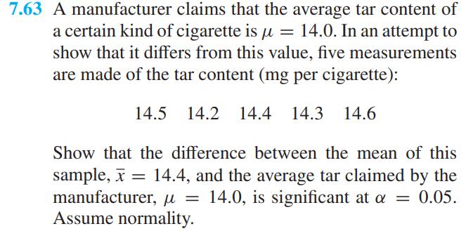
With reference to Exercise 7.63, construct a \(99 \%\) confidence interval for the variance of the population sampled.Data From Exercise 7.63 7.63 A manufacturer claims that the average tar content of a certain kind of cigarette is = 14.0. In an attempt to show that it differs from this value,
Use the value \(s\) obtained in Exercise 9.3 to construct a \(98 \%\) confidence interval for \(\sigma\), measuring the actual variability in the hardness of Alloy 1.Data From Exercise 9.3Data From Exercise 8.13 9.3 Use the data of part (a) of Exercise 8.13 to estimate for the Brinell hardness of
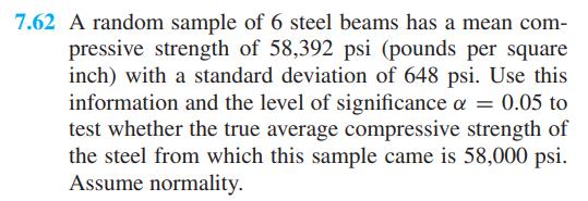
With reference to Exercise 7.62, test the null hypothesis \(\sigma=600\) psi for the compressive strength of the given kind of steel against the alternative hypothesis \(\sigma>600\) psi. Use the 0.05 level of significance.Data From Exercise 7.62 7.62 A random sample of 6 steel beams has a mean
If 15 determinations of the purity of gold have a standard deviation of 0.0015 , test the null hypothesis that \(\sigma=0.002\) for such determinations. Use the alternative hypothesis \(\sigma eq 0.002\) and the level of significance \(\alpha=0.05\).
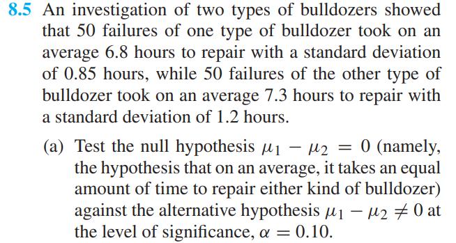
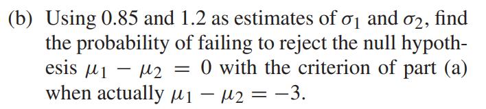
With reference to Exercise 8.5, test the null hypothesis that \(\sigma=0.75\) hours for the time that is required for repairs of the second type of bulldozer against the alternative hypothesis that \(\sigma>0.75\) hours. Use the 0.10 level of significance and assume normality.Data From Exercise
Use the 0.01 level of significance to test the null hypothesis that \(\sigma=0.015\) inch for the diameters of certain bolts against the alternative hypothesis that\(\sigma eq 0.015\) inch, given that a random sample of size 15 yielded \(s^{2}=0.00011\).
Playing 10 rounds of golf on his home course, a golf professional averaged 71.3 with a standard deviation of 2.64 .(a) Test the null hypothesis that the consistency of his game on his home course is actually measured by \(\sigma=2.40\), against the alternative hypothesis that he is less consistent.
The fire department of a city wants to test the null hypothesis that \(\sigma=10\) minutes for the time it takes a fire truck to reach a fire site against the alternative hypothesis \(\sigma eq 10\) minutes. What can it conclude at the 0.05 level of significance if a random sample of size \(n=48\)
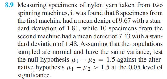
Explore the use of the two sample \(t\) test in Exercise 8.9 by testing the null hypothesis that the two populations have equal variances. Use the 0.02 level of significance.Data From Exercise 8.9 8.9 Measuring specimens of nylon yarn taken from two spinning machines, it was found that 8
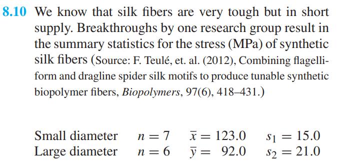
With reference to Exercise 8.10, use the 0.10 level of significance to test the assumption that the two populations have equal variances.Data From Exercise 8.10 8.10 We know that silk fibers are very tough but in short supply. Breakthroughs by one research group result in the summary statistics for
Two different computer processors are compared by measuring the processing speed for different operations performed by computers using the two processors. If 12 measurements with the first processor had a standard deviation of \(0.1 \mathrm{GHz}\) and 16 measurements with the second processor had a
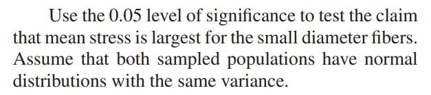
With reference to Exercise 8.6, where we had \(n_{1}=\) \(40, n_{2}=30, s_{1}=15.2\), and \(s_{2}=18.7\), use the 0.05 level of significance to test the claim that there is a greater variability in the number of cars which make left turns approaching from the south between 4 P.M. and 6 P.M. at the
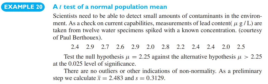
With reference to Example 20, Chapter 7, construct a 95% confidence interval for the true standard deviation of the lead content.Data From Example 20 EXAMPLE 20 At test of a normal population mean Scientists need to be able to detect small amounts of contaminants in the environ- ment. As a check on
If 44 measurements of the refractive index of a diamond have a standard deviation of 2.419 , construct a 95% confidence interval for the true standard deviation of such measurements. What assumptions did you make about the population?
Past data indicate that the variance of measurements made on sheet metal stampings by experienced quality-control inspectors is 0.18 (inch) \({ }^{2}\). Such measurements made by an inexperienced inspector could have too large a variance (perhaps because of inability to read instruments properly)
Thermal resistance tests on 13 samples of Enterococcus hirae, present in milk, yield the following results in degrees Celsius:Another set of seven samples of milk was tested after pasteurization to determine whether thermal resistance had been increased by pasteurization of milk, with the following
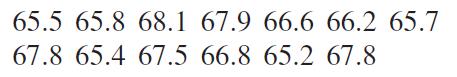
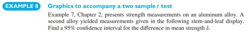
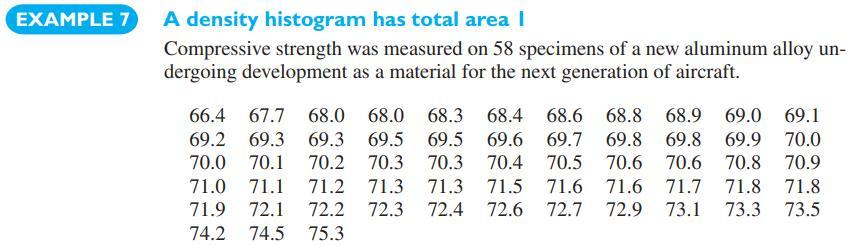
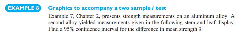
With reference to the Example 8, Chapter 8, test the equality of the variances for the two aluminum alloys. Use the 0.02 level of significance.Data From Example 8 EXAMPLE 8 Graphics to accompany a two sample t test Example 7, Chapter 2, presents strength measurements on an aluminum alloy. A second
With reference to the Example 8, Chapter 8, find a 98% confidence interval for the ratio of variances of the two aluminum alloys.Data From Example 8 EXAMPLE 8 Graphics to accompany a two sample / test Example 7, Chapter 2, presents strength measurements on an aluminum alloy. A second alloy yielded
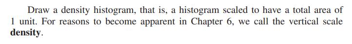
MINITAB calculation of \(t_{\alpha}, \chi_{v}^{2}\), and \(F_{\alpha}\)The software finds percentiles, so to obtain \(F_{\alpha}\), we first convert from \(\alpha\) to \(1-\alpha\). We illustrate with the calculation of \(F_{0.025}(4,7)\), where \(1-0.025=0.975\).Output:F distribution with \(4
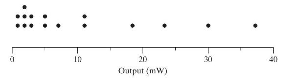
A bioengineering company manufactures a device for externally measuring blood flow. Measurements of the electrical output (milliwatts) on a sample of 16 units yields the data plotted in Figure 9.5.(a) Should you report the 95% confidence interval for \(\sigma\) using the formula in this chapter?
An inspector examines every twentieth piece coming off an assembly line. List some of the conditions under which this method of sampling might not yield a random sample.
Large maps are printed on a plotter and rolled up. The supervisor randomly selects 12 printed maps and unfolds a part of each map to verify the quality of the printing. List one condition under which this method of sampling might not yield a random sample.
Explain why the following will not lead to random samples from the desired populations.(a) To determine what the average person spends on a vacation, a market researcher interviews passengers on a luxury cruise.(b) To determine the average income of its graduates 10 years after graduation, the
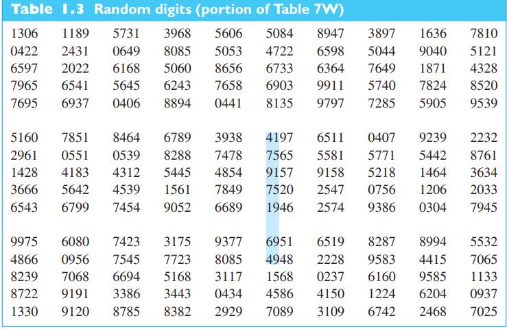
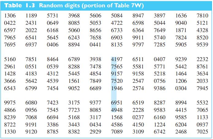
A market research organization wants to try a new product in 8 of 50 states. Use Table 7W or software to make this selection.Data From Table 7W Table 1.3 Random digits (portion of Table 7W) 1306 1189 5731 3968 5606 0422 2431 0649 8085 5053 5084 4722 6598 8947 3897 1636 7810 5044 9040 5121 6597 2022
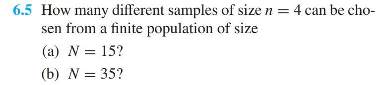
How many different samples of size \(n=4\) can be chosen from a finite population of size(a) \(N=15\) ?(b) \(N=35\) ?
With reference to Exercise 6.5, what is the probability of each sample in part(a) and the probability of each sample in part(b) if the samples are to be random?Data From Exercise 6.5 6.5 How many different samples of size n = 4 can be cho- sen from a finite population of size (a) N = 15? (b) N = 35?
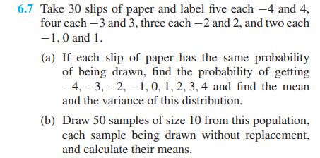
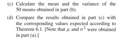
Take 30 slips of paper and label five each -4 and 4, four each -3 and 3 , three each -2 and 2 , and two each \(-1,0\) and 1 .(a) If each slip of paper has the same probability of being drawn, find the probability of getting \(-4,-3,-2,-1,0,1,2,3,4\) and find the mean and the variance of this
Repeat Exercise 6.7, but select each sample with replacement; that is, replace each slip of paper and reshuffle before the next one is drawn.Data From Exercise 6.7 6.7 Take 30 slips of paper and label five each -4 and 4, four each-3 and 3, three each-2 and 2, and two each -1,0 and 1. (a) If each
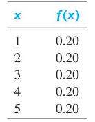
Given an infinite population whose distribution is given bylist the 25 possible samples of size 2 and use this list to construct the distribution of \(\bar{X}\) for random samples of size 2 from the given population. Verify that the mean and the variance of this sampling distribution are identical
Suppose that we convert the 50 samples referred to on page 197 into 25 samples of size \(n=20\) by combining the first two, the next two, and so on. Find the means of these samples and calculate their mean and their standard deviation. Compare this mean and this standard deviation with the
When we sample from an infinite population, what happens to the standard error of the mean if the sample size is(a) increased from 40 to 1,000 ?(b) decreased from 256 to 65 ?(c) increased from 225 to 1,225 ?(d) decreased from 450 to 18 ?
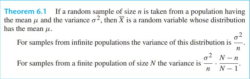
What is the value of the finite population correction factor in the formula for \(\sigma_{\bar{X}}^{2}\) when(a) \(n=8\) and \(N=640\) ?(b) \(n=100\) and \(N=8,000\) ?(c) \(n=250\) and \(N=20,000\) ?
For large sample size \(n\), verify that there is a \(50-50\) chance that the mean of a random sample from an infinite population with the standard deviation \(\sigma\) will differ from \(\mu\) by less than \(0.6745 \cdot \sigma / \sqrt{n}\). It has been the custom to refer to this quantity as the
The mean of a random sample of size \(n=25\) is used to estimate the mean of an infinite population that has standard deviation \(\sigma=2.4\). What can we assert about the probability that the error will be less than 1.2 , if we use(a) Chebyshev's theorem;(b) the central limit theorem?
Engine bearings depend on a film of oil to keep shaft and bearing surfaces separated. Insufficient lubrication causes bearings to be overloaded. The insufficient lubrication can be modeled as a random variable having mean 0.6520 ml and standard deviation 0.0125 ml.The sample mean of insufficient
A wire-bonding process is said to be in control if the mean pull strength is 10 pounds. It is known that the pull-strength measurements are normally distributed with a standard deviation of 1.5 pounds. Periodic random samples of size 4 are taken from this process and the process is said to be "out
If the distribution of scores of all students in an examination has a mean of 296 and a standard deviation of 14 , what is the probability that the combined gross score of 49 randomly selected students is less than 14,250?
If \(X\) is a continuous random variable and \(Y=X-\mu\), show that \(\sigma_{Y}^{2}=\sigma_{X}^{2}\).
Prove that \(\mu_{\bar{X}}=\mu\) for random samples from discrete (finite or countably infinite) populations.
The tensile strength (1,000 psi) of a new composite can be modeled as a normal distribution. A random sample of size 25 specimens has mean \(\bar{x}=45.3\) and standard deviation s=7.9. Does this information tend to support or refute the claim that the mean of the population is 40.5 ?
The following is the time taken (in hours) for the delivery of 8 parcels within a city: 28,32,20,26, 42,40,28, and 30 . Use these figures to judge the reasonableness of delivery services when they say it takes 30 hours on average to deliver a parcel within the city.
The process of making concrete in a mixer is under control if the rotations per minute of the mixer has a mean of 22 rpm. What can we say about this process if a sample of 20 of these mixers has a mean rpm of 22.75 rpm and a standard deviation of 3 rpm?
Engine bearings depend on a film of oil to keep shaft and bearing surfaces separated. Samples are regularly taken from production lines and each bearing in a sample is tested to measure the thickness of the oil film. After many samples, it is concluded that the population is normal. The variance is
A random sample of 15 observations is taken from a normal population having variance \(\sigma^{2}=90.25\). Find the approximate probability of obtaining a sample standard deviation between 7.25 and 10.75 .
If independent random samples of size \(n_{1}=n_{2}=8\) come from normal populations having the same variance, what is the probability that either sample variance will be at least 7 times as large as the other?
Find the values of(a) \(F_{0.95}\) for 15 and 12 degrees of freedom;(b) \(F_{0.99}\) for 5 and 20 degrees of freedom.
The chi square distribution with 4 degrees of freedom is given by\[f(x)= \begin{cases}\frac{1}{4} \cdot x \cdot e^{-x / 2} & x>0 \\ 0 & x \leq 0\end{cases}\]Find the probability that the variance of a random sample of size 5 from a normal population with \(\sigma=15\) will exceed 180.
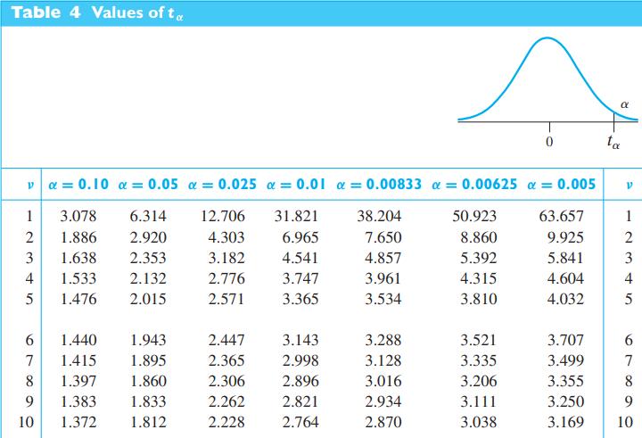
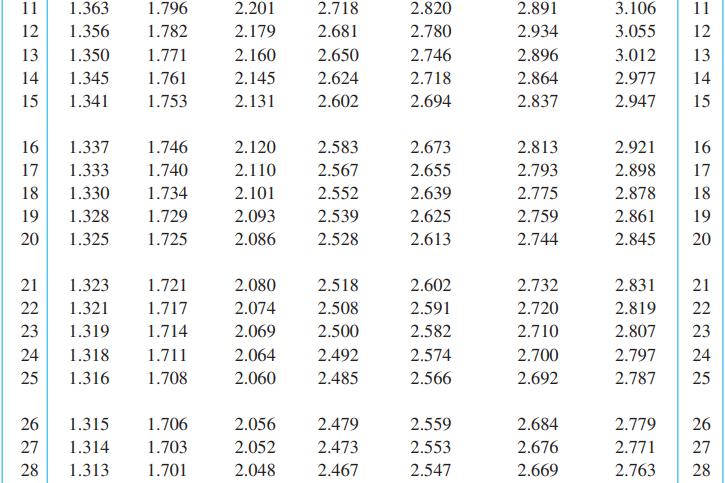
The \(t\) distribution with 1 degree of freedom is given by\[f(t)=\frac{1}{\pi}\left(1+t^{2}\right)^{-1} \quad-\inftyVerify the value given for \(t_{0.05}\) for \(v=1\) in Table 4 .Data From Table 4 Table 4 Values of ta 0 ta = 0.10 = 0.05 = 0.025 = 0.01 =0.00833 a = 0.00625 = 0.005 1 3.078.
The \(F\) distribution with 4 and 4 degrees of freedom is given by\[f(F)= \begin{cases}6 F(1+F)^{-4} & F>0 \\ 0 & F \leq 0\end{cases}\]If random samples of size 5 are taken from two normal populations having the same variance, find the probability that the ratio of the larger to the smaller sample
Let \(Z_{1}, \ldots, Z_{5}\) be independent and let each have a standard normal distribution.(a) Specify the distribution of \(Z_{2}^{2}+Z_{3}^{2}+Z_{4}^{2}+Z_{5}^{2}\).(b) Specify the distribution of \[\frac{Z_{1}}{\sqrt{\frac{Z_{2}^{2}+Z_{3}^{2}+Z_{4}^{2}+Z_{5}^{2}}{4}}}\]
Let \(Z_{1}, \ldots, Z_{6}\) be independent and let each have a standard normal distribution. Specify the distribution of\[\frac{Z_{1}-Z_{2}}{\sqrt{\frac{Z_{3}^{2}+Z_{4}^{2}+Z_{5}^{2}+Z_{6}^{2}}{8}}}\]
Let \(Z_{1}, \ldots, Z_{7}\) be independent and let each have a standard normal distribution.(a) Specify the distribution of \(Z_{1}^{2}+Z_{2}^{2}+Z_{3}^{2}+Z_{4}^{2}\).(b) Specify the distribution of \(Z_{5}^{2}+Z_{6}^{2}+Z_{7}^{2}\).(c) Specify the distribution of the sum of variables in part (a)
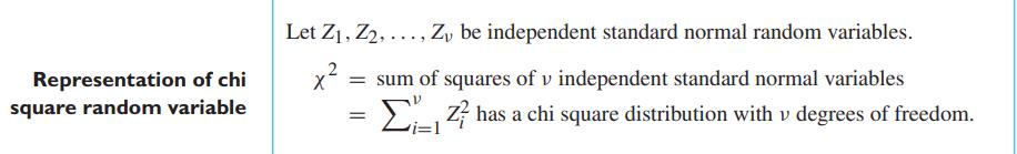
Let the chi square variables \(\chi_{1}^{2}\), with \(v_{1}\) degrees of freedom, and \(\chi_{2}^{2}\), with \(v_{2}\) degrees of freedom, be independent. Establish the result on page 211, that their sum is a chi square variable with \(v_{1}+v_{2}\) degrees of freedom. Representation of chi square
Let \(X_{1}, X_{2}, \ldots, X_{8}\) be 8 independent random variables. Find the moment generating function\[M_{\sum X_{i}}(t)=E\left(e^{t\left(X_{1}+X_{2}+\cdots+X_{8}\right)}\right)\]of the sum when \(X_{i}\) has a Poisson distribution with mean(a) \(\lambda_{i}=0.5\)(b) \(\lambda_{i}=0.04\)
Let \(X_{1}, X_{2}, \ldots, X_{5}\) be 5 independent random variables. Find the moment generating function\[M_{\sum X_{i}}(t)=E\left(e^{t\left(X_{1}+X_{2}+\cdots+X_{5}\right)}\right)\]of the sum when \(X_{i}\) has a gamma distribution with \(\alpha_{i}=2 i\) and \(\beta_{i}=2\).
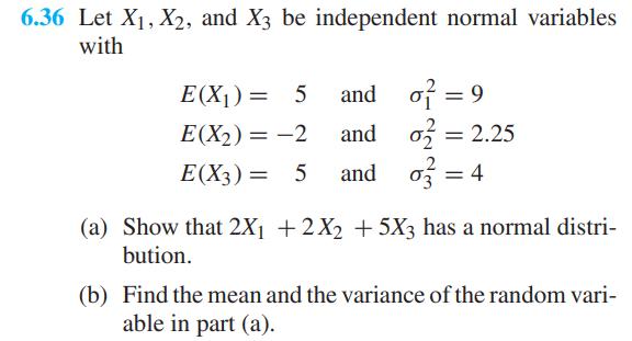
Let \(X_{1}, X_{2}\), and \(X_{3}\) be independent normal variables with\[\begin{array}{lll}E\left(X_{1}\right)=5 & \text { and } & \sigma_{1}^{2}=9 \\E\left(X_{2}\right)=-2 & \text { and } & \sigma_{2}^{2}=2.25 \\E\left(X_{3}\right)=5 & \text { and } & \sigma_{3}^{2}=4\end{array}\](a) Show that
Refer to Exercise 6.36.(a) Show that \(2 X_{1}-X_{2}-4 X_{3}-12\) has a normal distribution.(b) Find the mean and variance of the random variable in part (a).Data From Exercise 6.36 6.36 Let X1, X2, and X3 be independent normal variables with E(X1)= 5 and = 9 E(X2)=-2 and = 2.25 E(X3) = 5 and =
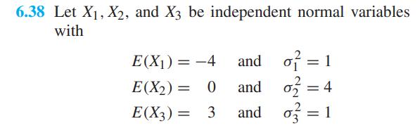
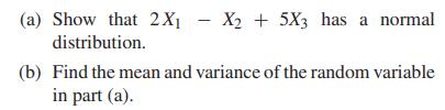
Let \(X_{1}, X_{2}\), and \(X_{3}\) be independent normal variables with\[\begin{array}{lll}E\left(X_{1}\right)=-4 & \text { and } & \sigma_{1}^{2}=1 \\E\left(X_{2}\right)=0 & \text { and } & \sigma_{2}^{2}=4 \\E\left(X_{3}\right)=3 & \text { and } & \sigma_{3}^{2}=1\end{array}\](a) Show that \(2
Refer to Exercise 6.38.(a) Show that \(7 X_{1}+X_{2}-2 X_{3}+7\) has a normal distribution.(b) Find the mean and variance of the random variable in part (a).Data From Exercise 6.38 6.38 Let X1, X2, and X3 be independent normal variables with E(X1)=-4 and = 1 o E(X2) = 0 and = 4 E(X3) = 3 and = 1
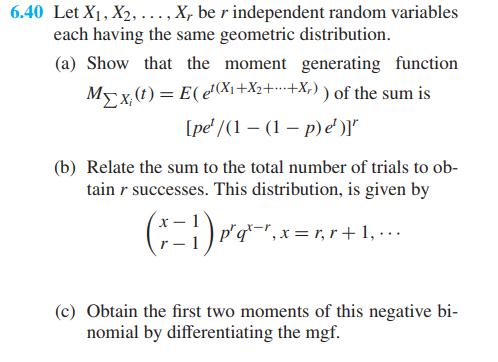
Let \(X_{1}, X_{2}, \ldots, X_{r}\) be \(r\) independent random variables each having the same geometric distribution.(a) Show that the moment generating function \(M_{\sum X_{i}}(t)=E\left(e^{t\left(X_{1}+X_{2}+\cdots+X_{r}\right)}\right)\) of the sum is\[\left[p e^{t} /\left(1-(1-p)
Refer to Exercise 6.40. Let \(X_{1}, X_{2}, \ldots, X_{n}\) be \(n\) independent random variables each having a negative binomial distribution with success probability \(p\) but where \(X_{i}\) has parameter \(r_{i}\).(a) Show that the \(\operatorname{mgf} M_{\sum
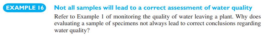
Referring to Example 16, verify that\[g(y)=\frac{1}{\sqrt{2 \pi}} y^{-1 / 2} e^{-y / 2}\]Data From Example 16 EXAMPLE 16 Not all samples will lead to a correct assessment of water quality Refer to Example 1 of monitoring the quality of water leaving a plant. Why does evaluating a sample of
Use the distribution function method to obtain the density of \(Z^{3}\) when \(Z\) has a standard normal distribution.
Use the distribution function method to obtain the density of \(1-e^{-X}\) when \(X\) has the exponential distribution with \(\beta=1\).
Use the distribution function method to obtain the density of \(\ln (X)\) when \(X\) has the exponential distribution with \(\beta=1\).
Use the transformation method to obtain the density of \(X^{3}\) when \(X\) has density \(f(x)=1.5 X\) for \(0
Use the transformation method to obtain the distribution of \(-\ln (X)\) when \(X\) has the uniform distribution on \((0,1)\).
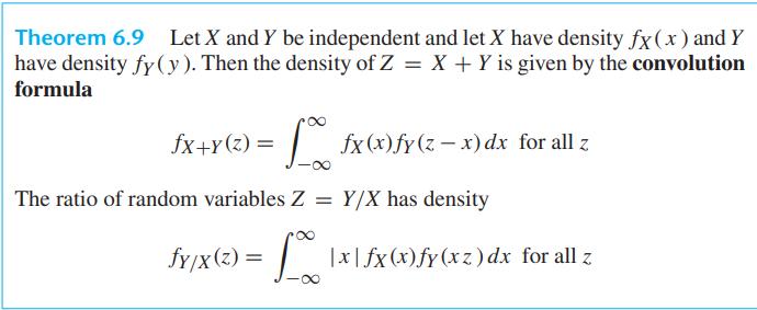
Use the convolution formula, Theorem 6.9, to obtain the density of \(X+Y\) when \(X\) and \(Y\) are independent and each has the exponential distribution with \(\beta=1\).Data From Theorem 6.9 Theorem 6.9 Let X and Y be independent and let X have density fx(x) and Y have density fy (y). Then the
Use the transformation method, Theorem 6.9, to obtain the distribution of the ratio \(Y / X\) when when \(X\) and \(Y\) are independent and each has the same gamma distribution.Data From Theorem 6.9 Theorem 6.9 Let X and Y be independent and let X have density fx(x) and Y have density fy (y). Then
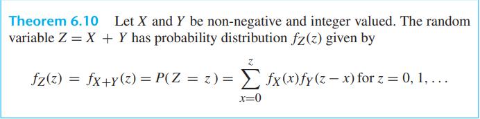
Use the discrete convolution formula, Theorem 6.10, to obtain the probability distribution of \(X+Y\) when \(X\) and \(Y\) are independent and each has the uniform distribution on \(\{0,1,2\}\).Data From Theorem 6.10 Theorem 6.10 Let X and Y be non-negative and integer valued. The random variable Z
The panel for a national science fair wishes to select 10 states from which a student representative will be chosen at random from the students participating in the state science fair.(a) Use Table 7W or software to select the 10 states.(b) Does the total selection process give each student who
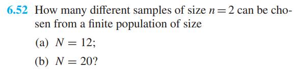
How many different samples of size \(n=2\) can be chosen from a finite population of size(a) \(N=12\);(b) \(N=20\) ?
With reference to Exercise 6.52, what is the probability of choosing each sample in part(a) and the probability of choosing each sample in part (b), if the samples are to be random?Data From Exercise 6.52 6.52 How many different samples of size n = 2 can be cho- sen from a finite population of size
Referring to Exercise 6.52, find the value of the finite population correction factor in the formula for \(\sigma_{\bar{X}}^{2}\) for part(a) and part (b).Data From Exercise 6.52 6.52 How many different samples of size n = 2 can be cho- sen from a finite population of size (a) N = 12; (b) N = 20?
The time to check out and process payment information at an office supplies Web site can be modeled as a random variable with mean \(\mu=63\) seconds and variance \(\sigma^{2}=81\). If the sample mean \(\bar{X}\) will be based on a random sample of \(n=36\) times, what can we assert about the
The number of pieces of mail that a department receives each day can be modeled by a distribution having mean 44 and standard deviation 8 . For a random sample of 35 days, what can be said about the probability that the sample mean will be less than 40 or greater than 48 using(a) Chebyshev's
If measurements of the elasticity of a fabric yarn can be looked upon as a sample from a normal population having a standard deviation of 1.8 , what is the probability that the mean of a random sample of size 26 will be less elastic by 0.63 ?
Adding graphite to iron can improve its ductile qualities. If measurements of the diameter of graphite spheres within an iron matrix can be modeled as a normal distribution having standard deviation 0.16 , what is the probability that the mean of a sample of size 36 will differ from the population
If 2 independent random samples of size \(n_{1}=31\) and \(n_{2}=11\) are taken from a normal population, what is the probability that the variance of the first sample will be at least 2.7 times as large as the variance of the second sample?
If 2 independent samples of sizes \(n_{1}=26\) and \(n_{2}=8\) are taken from a normal population, what is the probability that the variance of the second sample will be at least 2.4 times the variance of the first sample?
When we sample from an infinite population, what happens to the standard error of the mean if the sample size is(a) increased from 100 to 200 ;(b) increased from 200 to 300 ;(c) decreased from 360 to 90 ?
A traffic engineer collects data on traffic flow at a busy intersection during the rush hour by recording the number of westbound cars that are waiting for a green light. The observations are made for each light change. Explain why this sampling technique will not lead to a random sample.
Explain why the following may not lead to random samples from the desired population:(a) To determine the mix of animals in a forest, a forest officer records the animals observed after each interval of 2 minutes.(b) To determine the quality of print, an observer observes the quality of the first
Several pickers are each asked to gather 30 ripe apples and put them in a bag.(a) Would you expect all of the bags to weigh the same? For one bag, let \(X_{1}\) be the weight of the first apple, \(X_{2}\) the weight of the second apple, and so on. Relate the weight of this bag,\[\sum_{i=1}^{30}
A construction engineer collected data from some construction sites on the quantity of gravel (in metric tons) used in mixing concrete. The quantity of gravel for n=24 sites4861 5158 8642 2896 7654 9891 8381 6215 1116 7918 2313
An industrial engineer collected data on the labor time required to produce an order of automobile mufflers using a heavy stamping machine. The data on times (hours) for \(n=52\) orders of different parts\(\begin{array}{lllllllllll}2.15 & 2.27 & 0.99 & 0.63 & 2.45 & 1.30 &
The manufacture of large liquid crystal displays (LCD's) is difficult. Some defects are minor and can be removed; others are unremovable. The number of unremovable defects, for each of \(n=45\) displays (Courtesy of Shiyu Zhou)has \(\bar{x}=2.467\) and \(s=3.057\) unremovable defects. What can one
In a study of automobile collision insurance costs, a random sample of 80 body repair costs for a particular kind of damage had a mean of \(\$ 472.36\) and a standard deviation of \(\$ 62.35\). If \(\bar{x}=\$ 472.36\) is used as a point estimate of the true average repair cost of this kind of
Refer to Example 8. How large a sample will we need in order to assert with probability 0.95 that the sample mean will not differ from the true mean by more than 1.5. (replacing \(\sigma\) by \(s\) is reasonable here because the estimate is based on a sample of size eighteen.)Data From Example
The dean of a college wants to use the mean of a random sample to estimate the average amount of time students take to get from one class to the next, and she wants to be able to assert with \(99 \%\) confidence that the error is at most 0.25 minute. If it can be presumed from experience that
An effective way to tap rubber is to cut a panel in the rubber tree's bark in vertical spirals. In a pilot process, an engineer measures the output of latex from such cuts. Eight cuts on different trees produced latex (in liters) in a week\[\begin{array}{llllllll}26.8 & 32.5 & 29.7 & 24.6 & 31.5 &
To monitor complex chemical processes, chemical engineers will consider key process indicators, which may be just yield but most often depend on several quantities. Before trying to improve a process, \(n=9\) measurements were made on a key performance indicator.\[\begin{array}{lllllllll}123 & 106
With reference to the previous exercise, assume that the key performance indicator has a normal distribution and obtain a \(95 \%\) confidence interval for the true value of the indicator.
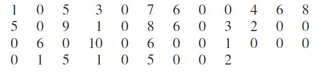
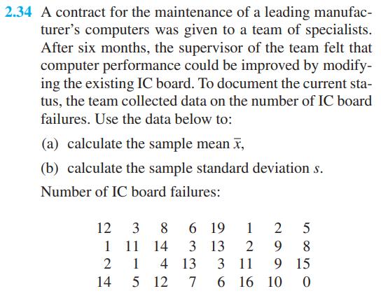
Refer to Exercise 2.34, page 46, concerning the number for board failures for \(n=32\) integrated circuits (IC). A computer calculates \(\bar{x}=7.6563\) and \(s=5.2216\). Obtain a 95\% confidence interval for the mean IC board failures.Data From Exercise 2.34 2.34 A contract for the maintenance of
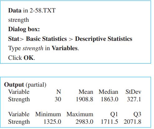
Refer to the \(2 \times 4\) lumber strength data in Exercise 2.58, page 48. According to the computer output, a sample of \(n=30\) specimens had \(\bar{x}=1908.8\) and \(s=\) 327.1. Find a \(95 \%\) confidence interval for the population mean strength.Data From Exercise 2.58 2.58 Modern computer
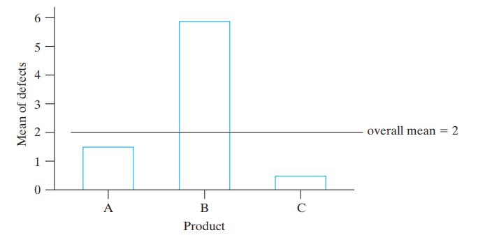
Refer to the data on page 50, on the number of defects per board for Product B. Obtain a 95% confidence interval for the population mean number of defects per board. 5 Mean of defects 2 3 + 1 19 6 0 A B C Product overall mean = 2
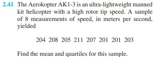
With reference to the thickness measurements in Exercise 2.41 , page 47 , obtain a \(95 \%\) confidence interval for the mean thickness.Data From Exercise 2.41 2.41 The Aerokopter AK1-3 is an ultra-lightweight manned kit helicopter with a high rotor tip speed. A sample of 8 measurements of speed,
Ten bearings made by a certain process have a mean diameter of \(0.5060 \mathrm{~cm}\) and a standard deviation of \(0.0040 \mathrm{~cm}\). Assuming that the data may be looked upon as a random sample from a normal population, construct a 95\% confidence interval for the actual average diameter of

Showing 6000 - 6100 of 7136

First
54
55
56
57
58
59
60
61
62
63
64
65
66
67
68
Last

Step by Step Answers

Services

Sitemap
Fun
Definitions
Become Tutor
Used Textbooks
Study Help Categories
Recent Questions
Expert Questions
Campus Wear
Sell Your Books

Company Info

Security
Copyrights
Privacy Policy
Terms & Conditions
SolutionInn Fee
Scholarship
Online Quiz
Give Feedback, Get Rewards

Get In Touch

About Us
Contact Us
Career
Jobs
FAQ
Student Discount
Campus Ambassador

Secure Payment

Download Our App

© 2026 SolutionInn. All Rights Reserved